← return to practice.dsc10.com
These problems are taken from past quizzes and exams. Work on them
on paper, since the quizzes and exams you take in this
course will also be on paper.
We encourage you to complete these
problems during discussion section. Solutions will be made available
after all discussion sections have concluded. You don’t need to submit
your answers anywhere.
Note: We do not plan to cover all of
these problems during the discussion section; the problems we don’t
cover can be used for extra practice.
Researchers from the San Diego Zoo, located within Balboa Park, collected physical measurements of several species of penguins in a region of Antarctica.
One piece of information they tracked for each of 330 penguins was its mass in grams. The average penguin mass is 4200 grams, and the standard deviation is 840 grams.
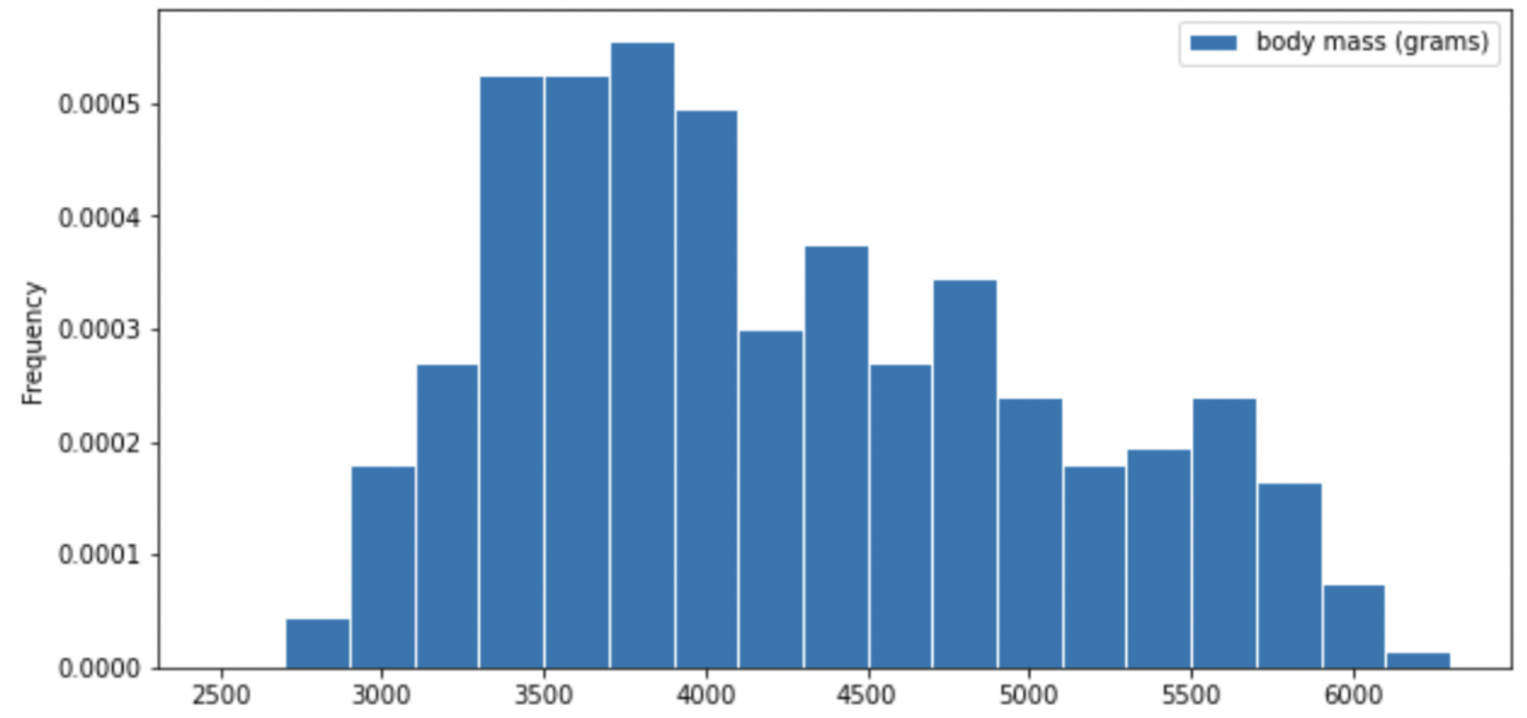
Consider the histogram of mass below.

Select the true statement below.
The median mass of penguins is larger than the average mass of penguins
The median mass of penguins is roughly equal to the average mass of penguins (within 50 grams)
The median mass of penguins is less than the average mass of penguins
It is impossible to determine the relationship between the median and average mass of penguins just by looking at the above histogram
Answer: The median mass of penguins is less than the average mass of penguins
This is a distribution that is skewed to the right, so mean is greater than median.
The average score on this problem was 87%.
For your convenience, we show the histogram of mass again below.

Recall, there are 330 penguins in our dataset. Their average mass is 4200 grams, and the standard deviation of mass is 840 grams.
Per Chebyshev’s inequality, at least what percentage of penguins have a mass between 3276 grams and 5124 grams? Input your answer as a percentage between 0 and 100, without the % symbol. Round to three decimal places.
Answer: 17.355
Recall, Chebyshev’s inequality states that No matter what the shape of the distribution is, the proportion of values in the range “average ± z SDs” is at least 1 - \frac{1}{z^2}.
To approach the problem, we’ll start by converting 3276 grams and 5124 grams to standard units. Doing so yields \frac{3276 - 4200}{840} = -1.1, similarly, \frac{5124 - 4200}{840} = 1.1. This means that 3276 is 1.1 standard deviations below the mean, and 5124 is 1.1 standard deviations above the mean. Thus, we are calculating the proportion of values in the range “average ± 1.1 SDs”.
When z = 1.1, we have 1 - \frac{1}{z^2} = 1 - \frac{1}{1.1^2} \approx 0.173553719, which as a percentage rounded to three decimal places is 17.355\%.
The average score on this problem was 76%.
Per Chebyshev’s inequality, at least what percentage of penguins have a mass between 1680 grams and 5880 grams?
50%
55.5%
65.25%
68%
75%
88.8%
95%
Answer: 75%
Recall: proportion with z SDs of the mean
| Percent in Range | All Distributions (via Chebyshev’s Inequality) | Normal Distributions |
|---|---|---|
| \text{average} \pm 1 \ \text{SD} | \geq 0\% | \approx 68\% |
| \text{average} \pm 2\text{SDs} | \geq 75\% | \approx 95\% |
| \text{average} \pm 3\text{SDs} | \geq 88\% | \approx 99.73\% |
To approach the problem, we’ll start by converting 3276 grams and 5124 grams to standard units. Doing so yields \frac{1680 - 4200}{840} = -3, similarly, \frac{5880 - 4200}{840} = 2. This means that 1680 is 3 standard deviations below the mean, and 5880 is 2 standard deviations above the mean.
Proportion of values in [-3 SUs, 2 SUs] >= Proportion of values in [-2 SUs, 2 SUs] >= 75% (Since we cannot assume that the distribution is normal, we look at the All Distributions (via Chebyshev’s Inequality) column for proportion).
Thus, at least 75% of the penguins have a mass between 1680 grams and 5880 grams.
The average score on this problem was 72%.
The distribution of mass in grams is not roughly normal. Is the distribution of mass in standard units roughly normal?
Yes
No
Impossible to tell
Answer: No
The shape of the distribution does not change since we are scaling the x values for all data.
The average score on this problem was 60%.
Suppose boot_means is an array of the resampled means.
Fill in the blanks below so that [left, right] is a 68%
confidence interval for the true mean mass of penguins.
left = np.percentile(boot_means, __(a)__)
right = np.percentile(boot_means, __(b)__)
[left, right]
What goes in blank (a)? What goes in blank (b)?
Answer: (a) 16 (b) 84
Recall, np.percentile(array, p) computes the
pth percentile of the numbers in array. To
compute the 68% CI, we need to know the percentile of left tail and
right tail.
left percentile = (1-0.68)/2 = (0.32)/2 = 0.16 so we have 16th percentile
right percentile = 1-((1-0.68)/2) = 1-((0.32)/2) = 1-0.16 = 0.84 so we have 84th percentile
The average score on this problem was 94%.
Which of the following is a correct interpretation of this confidence interval? Select all that apply.
There is an approximately 68% chance that mean weight of all penguins in Antarctica falls within the bounds of this confidence interval.
Approximately 68% of penguin weights in our sample fall within the bounds of this confidence interval.
Approximately 68% of penguin weights in the population fall within the bounds of this interval.
If we created many confidence intervals using the same method, approximately 68% of them would contain the mean weight of all penguins in Antarctica.
None of the above
Answer: Option 4 (If we created many confidence intervals using the same method, approximately 68% of them would contain the mean weight of all penguins in Antarctica.)
Recall, what a k% confidence level states is that approximately k% of the time, the intervals you create through this process will contain the true population parameter.
In this question, our population parameter is the mean weight of all penguins in Antarctica. So 86% of the time, the intervals you create through this process will contain the mean weight of all penguins in Antarctica. This is the same as Option 4. However, it will be false if we state it in the reverse order (Option 1) since our population parameter is already fixed.
The average score on this problem was 81%.
An IKEA chair designer is experimenting with some new ideas for armchair designs. She has the idea of making the arm rests shaped like bell curves, or normal distributions. A cross-section of the armchair design is shown below.

This was created by taking the portion of the standard normal distribution from z=-4 to z=4 and adjoining two copies of it, one centered at z=0 and the other centered at z=8. Let’s call this shape the armchair curve.
Since the area under the standard normal curve from z=-4 to z=4 is approximately 1, the total area under the armchair curve is approximately 2.
Complete the implementation of the two functions below:
area_left_of(z) should return the area under the
armchair curve to the left of z, assuming
-4 <= z <= 12, andarea_between(x, y) should return the area under the
armchair curve between x and y, assuming
-4 <= x <= y <= 12.import scipy
def area_left_of(z):
'''Returns the area under the armchair curve to the left of z.
Assume -4 <= z <= 12'''
if ___(a)___:
return ___(b)___
return scipy.stats.norm.cdf(z)
def area_between(x, y):
'''Returns the area under the armchair curve between x and y.
Assume -4 <= x <= y <= 12.'''
return ___(c)___What goes in blank (a)?
Answer: z>4 or
z>=4
The body of the function contains an if statement
followed by a return statement, which executes only when
the if condition is false. In that case, the function
returns scipy.stats.norm.cdf(z), which is the area under
the standard normal curve to the left of z. When
z is in the left half of the armchair curve, the area under
the armchair curve to the left of z is the area under the
standard normal curve to the left of z because the left
half of the armchair curve is a standard normal curve, centered at 0. So
we want to execute the return statement in that case, but
not if z is in the right half of the armchair curve, since
in that case the area to the left of z under the armchair
curve should be more than 1, and scipy.stats.norm.cdf(z)
can never exceed 1. This means the if condition needs to
correspond to z being in the right half of the armchair
curve, which corresponds to z>4 or z>=4,
either of which is a correct solution.
The average score on this problem was 72%.
What goes in blank (b)?
Answer:
1+scipy.stats.norm.cdf(z-8)
This blank should contain the value we want to return when
z is in the right half of the armchair curve. In this case,
the area under the armchair curve to the left of z is the
sum of two areas:
z.Since the right half of the armchair curve is just a standard normal
curve that’s been shifted to the right by 8 units, the area under that
normal curve to the left of z is the same as the area to
the left of z-8 on the standard normal curve that’s
centered at 0. Adding the portion from the left half and the right half
of the armchair curve gives
1+scipy.stats.norm.cdf(z-8).
For example, if we want to find the area under the armchair curve to the left of 9, we need to total the yellow and blue areas in the image below.

The yellow area is 1 and the blue area is the same as the area under the standard normal curve (or the left half of the armchair curve) to the left of 1 because 1 is the point on the left half of the armchair curve that corresponds to 9 on the right half. In general, we need to subtract 8 from a value on the right half to get the corresponding value on the left half.
The average score on this problem was 54%.
What goes in blank (c)?
Answer:
area_left_of(y) - area_left_of(x)
In general, we can find the area under any curve between
x and y by taking the area under the curve to
the left of y and subtracting the area under the curve to
the left of x. Since we have a function to find the area to
the left of any given point in the armchair curve, we just need to call
that function twice with the appropriate inputs and subtract the
result.
The average score on this problem was 60%.
Suppose you have correctly implemented the function
area_between(x, y) so that it returns the area under the
armchair curve between x and y, assuming the
inputs satisfy -4 <= x <= y <= 12.
Note: You can still do this question, even if you didn’t know how to do the previous one.
What is the approximate value of
area_between(-2, 10)?
1.9
1.95
1.975
2
Answer: 1.95
The area we want to find is shown below in two colors. We can find the area in each half of the armchair curve separately and add the results.

For the yellow area, we know that the area within 2 standard deviations of the mean on the standard normal curve is 0.95. The remaining 0.05 is split equally on both sides, so the yellow area is 0.975.
The blue area is the same by symmetry so the total shaded area is 0.975*2 = 1.95.
Equivalently, we can use the fact that the total area under the armchair curve is 2, and the amount of unshaded area on either side is 0.025, so the total shaded area is 2 - (0.025*2) = 1.95.
The average score on this problem was 76%.
What is the approximate value of
area_between(0.37, 8.37)?
0.68
0.95
1
1.5
Answer: 1
The area we want to find is shown below in two colors.

As we saw in Problem 12.2, the point on the left half of the armchair curve that corresponds to 8.37 is 0.37. This means that if we move the blue area from the right half of the armchair curve to the left half, it will fit perfectly, as shown below.

Therefore the total of the blue and yellow areas is the same as the area under one standard normal curve, which is 1.
The average score on this problem was 76%.
Oren has a random sample of 200 dog prices in an array called
oren. He has also bootstrapped his sample 1,000 times and
stored the mean of each resample in an array called
boots.
In this question, assume that the following code has run:
a = np.mean(oren)
b = np.std(oren)
c = len(oren)What expression best estimates the population’s standard deviation?
b
b / c
b / np.sqrt(c)
b * np.sqrt(c)
Answer: b
The function np.std directly calculated the standard
deviation of array oren. Even though oren is
sample of the population, its standard deviation is still a pretty good
estimate for the standard deviation of the population because it is a
random sample. The other options don’t really make sense in this
context.
The average score on this problem was 57%.
Which expression best estimates the mean of boots?
0
a
(oren - a).mean()
(oren - a) / b
Answer: a
Note that a is equal to the mean of oren,
which is a pretty good estimator of the mean of the overall population
as well as the mean of the distribution of sample means. The other
options don’t really make sense in this context.
The average score on this problem was 89%.
What expression best estimates the standard deviation of
boots?
b
b / c
b / np.sqrt(c)
(a -b) / np.sqrt(c)
Answer: b / np.sqrt(c)
Note that we can use the Central Limit Theorem for this problem which
states that the standard deviation (SD) of the distribution of sample
means is equal to (population SD) / np.sqrt(sample size).
Since the SD of the sample is also the SD of the population in this
case, we can plug our variables in to see that
b / np.sqrt(c) is the answer.
The average score on this problem was 91%.
What is the dog price of $560 in standard units?
(560 - a) / b
(560 - a) / (b / np.sqrt(c))
(a - 560) / (b / np.sqrt(c))}
abs(560 - a) / b
abs(560 - a) / (b / np.sqrt(c))
Answer: (560 - a) / b
To convert a value to standard units, we take the value, subtract the
mean from it, and divide by SD. In this case that is
(560 - a) / b, because a is the mean of our
dog prices sample array and b is the SD of the dog prices
sample array.
The average score on this problem was 80%.
The distribution of boots is normal because of the
Central Limit Theorem.
True
False
Answer: True
True. The central limit theorem states that if you have a population and you take a sufficiently large number of random samples from the population, then the distribution of the sample means will be approximately normally distributed.
The average score on this problem was 91%.
If Oren’s sample was 400 dogs instead of 200, the standard deviation
of boots will…
Increase by a factor of 2
Increase by a factor of \sqrt{2}
Decrease by a factor of 2
Decrease by a factor of \sqrt{2}
None of the above
Answer: Decrease by a factor of \sqrt{2}
Recall that the central limit theorem states that the STD of the
sample distribution is equal to
(population STD) / np.sqrt(sample size). So if we increase
the sample size by a factor of 2, the STD of the sample distribution
will decrease by a factor of \sqrt{2}.
The average score on this problem was 80%.
If Oren took 4000 bootstrap resamples instead of 1000, the standard
deviation of boots will…
Increase by a factor of 4
Increase by a factor of 2
Decrease by a factor of 2
Decrease by a factor of 4
None of the above
Answer: None of the above
Again, from our formula given by the central limit theorem, the
sample STD doesn’t depend on the number of bootstrap resamples so long
as it’s “sufficiently large”. Thus increasing our bootstrap sample from
1000 to 4000 will have no effect on the std of boots
The average score on this problem was 74%.
Write one line of code that evaluates to the right endpoint of a 92% CLT-Based confidence interval for the mean dog price. The following expressions may help:
stats.norm.cdf(1.75) # => 0.96
stats.norm.cdf(1.4) # => 0.92Answer: a + 1.75 * b / np.sqrt(c)
Recall that a 92% confidence interval means an interval that consists
of the middle 92% of the distribution. In other words, we want to “chop”
off 4% from either end of the ditribution. Thus to get the right
endpoint, we want the value corresponding to the 96th percentile in the
mean dog price distribution, or
mean + 1.75 * (SD of population / np.sqrt(sample size) or
a + 1.75 * b / np.sqrt(c) (we divide by
np.sqrt(c) due to the central limit theorem). Note that the
second line of information that was given
stats.norm.cdf(1.4) is irrelavant to this particular
problem.
The average score on this problem was 48%.
From a population with mean 500 and standard deviation 50, you collect a sample of size 100. The sample has mean 400 and standard deviation 40. You bootstrap this sample 10,000 times, collecting 10,000 resample means.
Which of the following is the most accurate description of the mean of the distribution of the 10,000 bootstrapped means?
The mean will be exactly equal to 400.
The mean will be exactly equal to 500.
The mean will be approximately equal to 400.
The mean will be approximately equal to 500.
Answer: The mean will be approximately equal to 400.
The distribution of bootstrapped means’ mean will be approximately 400 since that is the mean of the sample and bootstrapping is taking many samples of the original sample. The mean will not be exactly 400 do to some randomness though it will be very close.
The average score on this problem was 54%.
Which of the following is closest to the standard deviation of the distribution of the 10,000 bootstrapped means?
400
40
4
0.4
Answer: 4
To find the standard deviation of the distribution, we can take the sample standard deviation S divided by the square root of the sample size. From plugging in, we get 40 / 10 = 4.
The average score on this problem was 51%.
Suppose you draw a sample of size 100 from a population with mean 50 and standard deviation 15. What is the probability that your sample has a mean between 50 and 53? Input the probability below, as a number between 0 and 1, rounded to two decimal places.
Answer: 0.48
This problem is testing our understanding of the Central Limit Theorem and normal distributions. Recall, the Central Limit Theorem tells us that the distribution of the sample mean is roughly normal, with the following characteristics:
\begin{align*} \text{Mean of Distribution of Possible Sample Means} &= \text{Population Mean} = 50 \\ \text{SD of Distribution of Possible Sample Means} &= \frac{\text{Population SD}}{\sqrt{\text{Sample Size}}} = \frac{15}{\sqrt{100}} = 1.5 \end{align*}
Given this information, it may be easier to express the problem as “We draw a value from a normal distribution with mean 50 and SD 1.5. What is the probability that the value is between 50 and 53?” Note that this probability is equal to the proportion of values between 50 and 53 in a normal distribution whose mean is 50 and 1.5 (since probabilities can be thought of as proportions).
In class, we typically worked with the standard normal distribution, in which the mean was 0, the SD was 1, and the x-axis represented values in standard units. Let’s convert the quantities of interest in this problem to standard units, keeping in mind that the mean and SD we’re using now are the mean and SD of the distribution of possible sample means, not of the population.
Now, our problem boils down to finding the proportion of values in a standard normal distribution that are between 0 and 2, or the proportion of values in a normal distribution that are in the interval [\text{mean}, \text{mean} + 2 \text{ SDs}].
From class, we know that in a normal distribution, roughly 95% of values are within 2 standard deviations of the mean, i.e. the proportion of values in the interval [\text{mean} - 2 \text{ SDs}, \text{mean} + 2 \text{ SDs}] is 0.95.
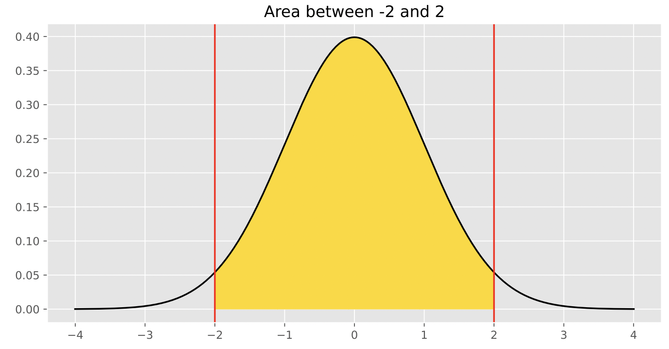
Since the normal distribution is symmetric about the mean, half of the values in this interval are to the right of the mean, and half are to the left. This means that the proportion of values in the interval [\text{mean}, \text{mean} + 2 \text{ SDs}] is \frac{0.95}{2} = 0.475, which rounds to 0.48, and thus the desired result is 0.48.
The average score on this problem was 48%.
The DataFrame apps contains application data for a
random sample of 1,000 applicants for a particular credit card from the
1990s. The "age" column contains the applicants’ ages, in
years, to the nearest twelfth of a year.
The credit card company that owns the data in apps,
BruinCard, has decided not to give us access to the entire
apps DataFrame, but instead just a random sample of 100
rows of apps called hundred_apps.
We are interested in estimating the mean age of all applicants in
apps given only the data in hundred_apps. The
ages in hundred_apps have a mean of 35 and a standard
deviation of 10.
Give the endpoints of the CLT-based 95% confidence interval for the
mean age of all applicants in apps, based on the data in
hundred_apps.
Answer: Left endpoint = 33, Right endpoint = 37
According to the Central Limit Theorem, the standard deviation of the distribution of the sample mean is \frac{\text{sample SD}}{\sqrt{\text{sample size}}} = \frac{10}{\sqrt{100}} = 1. Then using the fact that the distribution of the sample mean is roughly normal, since 95% of the area of a normal curve falls within two standard deviations of the mean, we can find the endpoints of the 95% CLT-based confidence interval as 35 - 2 = 33 and 35 + 2 = 37.
We can think of this as using the formula below: \left[\text{sample mean} - 2\cdot \frac{\text{sample SD}}{\sqrt{\text{sample size}}}, \: \text{sample mean} + 2\cdot \frac{\text{sample SD}}{\sqrt{\text{sample size}}} \right]. Plugging in the appropriate quantities yields [35 - 2\cdot\frac{10}{\sqrt{100}}, 35 - 2\cdot\frac{10}{\sqrt{100}}] = [33, 37].
The average score on this problem was 67%.
BruinCard reinstates our access to apps so that we can
now easily extract information about the ages of all applicants. We
determine that, just like in hundred_apps, the ages in
apps have a mean of 35 and a standard deviation of 10. This
raises the question of how other samples of 100 rows of
apps would have turned out, so we compute 10,000 sample means as follows.
    sample_means = np.array([])
    for i in np.arange(10000):
        sample_mean = apps.sample(100, replace=True).get("age").mean()
        sample_means = np.append(sample_means, sample_mean)
Which of the following three visualizations best depict the
distribution of sample_means?
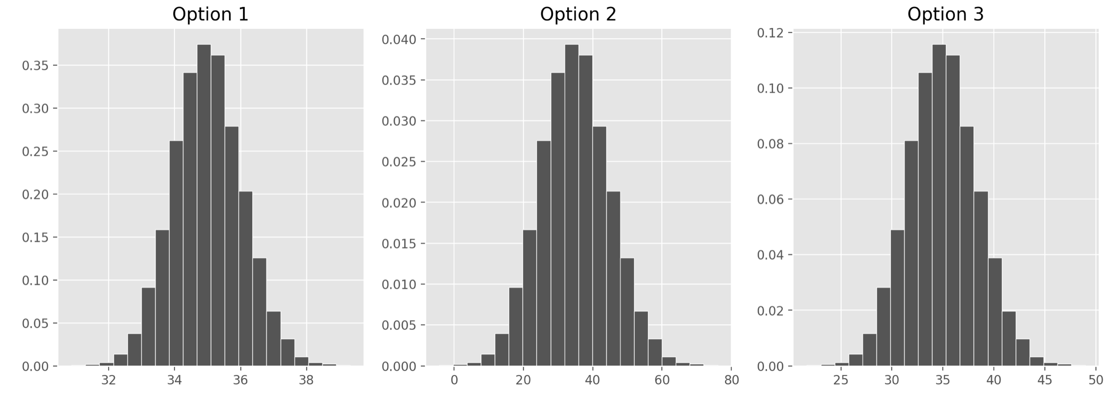
Answer: Option 1
As we found in the previous part, the distribution of the sample mean should have a standard deviation of 1. We also know it should be centered at the mean of our sample, at 35, but since all the options are centered here, that’s not too helpful. Only Option 1, however, has a standard deviation of 1. Remember, we can approximate the standard deviation of a normal curve as the distance between the mean and either of the inflection points. Only Option 1 looks like it has inflection points at 34 and 36, a distance of 1 from the mean of 35.
If you chose Option 2, you probably confused the standard deviation of our original sample, 10, with the standard deviation of the distribution of the sample mean, which comes from dividing that value by the square root of the sample size.
The average score on this problem was 57%.
Which of the following statements are guaranteed to be true? Select all that apply.
We used bootstrapping to compute sample_means.
The ages of credit card applicants are roughly normally distributed.
A CLT-based 90% confidence interval for the mean age of credit card applicants, based on the data in hundred apps, would be narrower than the interval you gave in part (a).
The expression np.percentile(sample_means, 2.5)
evaluates to the left endpoint of the interval you gave in part (a).
If we used the data in hundred_apps to create 1,000
CLT-based 95% confidence intervals for the mean age of applicants in
apps, approximately 950 of them would contain the true mean
age of applicants in apps.
None of the above.
Answer: A CLT-based 90% confidence interval for the
mean age of credit card applicants, based on the data in
hundred_apps, would be narrower than the interval you gave
in part (a).
Let’s analyze each of the options:
Option 1: We are not using bootstrapping to compute sample means
since we are sampling from the apps DataFrame, which is our
population here. If we were bootstrapping, we’d need to sample from our
first sample, which is hundred_apps.
Option 2: We can’t be sure what the distribution of the ages of
credit card applicants are. The Central Limit Theorem says that the
distribution of sample_means is roughly normally
distributed, but we know nothing about the population
distribution.
Option 3: The CLT-based 95% confidence interval that we calculated in part (a) was computed as follows: \left[\text{sample mean} - 2\cdot \frac{\text{sample SD}}{\sqrt{\text{sample size}}}, \text{sample mean} + 2\cdot \frac{\text{sample SD}}{\sqrt{\text{sample size}}} \right] A CLT-based 90% confidence interval would be computed as \left[\text{sample mean} - z\cdot \frac{\text{sample SD}}{\sqrt{\text{sample size}}}, \text{sample mean} + z\cdot \frac{\text{sample SD}}{\sqrt{\text{sample size}}} \right] for some value of z less than 2. We know that 95% of the area of a normal curve is within two standard deviations of the mean, so to only pick up 90% of the area, we’d have to go slightly less than 2 standard deviations away. This means the 90% confidence interval will be narrower than the 95% confidence interval.
Option 4: The left endpoint of the interval from part (a) was
calculated using the Central Limit Theorem, whereas using
np.percentile(sample_means, 2.5) is calculated empirically,
using the data in sample_means. Empirically calculating a
confidence interval doesn’t necessarily always give the exact same
endpoints as using the Central Limit Theorem, but it should give you
values close to those endpoints. These values are likely very similar
but they are not guaranteed to be the same. One way to see this is that
if we ran the code to generate sample_means again, we’d
probably get a different value for
np.percentile(sample_means, 2.5).
Option 5: The key observation is that if we used the data in
hundred_apps to create 1,000 CLT-based 95% confidence
intervals for the mean age of applicants in apps, all of
these intervals would be exactly the same. Given a sample, there is only
one CLT-based 95% confidence interval associated with it. In our case,
given the sample hundred_apps, the one and only CLT-based
95% confidence interval based on this sample is the one we found in part
(a). Therefore if we generated 1,000 of these intervals, either they
would all contain the parameter or none of them would. In order for a
statement like the one here to be true, we would need to collect 1,000
different samples, and calculate a confidence interval from each
one.
The average score on this problem was 49%.