← return to practice.dsc10.com
These problems are taken from past quizzes and exams. Work on them
on paper, since the quizzes and exams you take in this
course will also be on paper.
We encourage you to complete these
problems during discussion section. Solutions will be made available
after all discussion sections have concluded. You don’t need to submit
your answers anywhere.
Note: We do not plan to cover all of
these problems during the discussion section; the problems we don’t
cover can be used for extra practice.
Suppose we take a uniform random sample with replacement from a population, and use the sample mean as an estimate for the population mean. Which of the following is correct?
If we take a larger sample, our sample mean will be closer to the population mean.
If we take a smaller sample, our sample mean will be closer to the population mean.
If we take a larger sample, our sample mean is more likely to be close to the population mean than if we take a smaller sample.
If we take a smaller sample, our sample mean is more likely to be close to the population mean than if we take a larger sample.
Answer: If we take a larger sample, our sample mean is more likely to be close to the population mean than if we take a smaller sample.
Larger samples tend to give better estimates of the population mean than smaller samples. That’s because large samples are more like the population than small samples. We can see this in the extreme. Imagine a sample of 1 element from a population. The sample might vary a lot, depending on the distribution of the population. On the other extreme, if we sample the whole population, our sample mean will be exactly the same as the population mean.
Notice that the correct answer choice uses the words “is more likely to be close to” as opposed to “will be closer to.” We’re talking about a general phenomenon here: larger samples tend to give better estimates of the population mean than smaller samples. We cannot say that if we take a larger sample our sample mean “will be closer to” the population mean, since it’s always possible to get lucky with a small sample and unlucky with a large sample. That is, one particular small sample may happen to have a mean very close to the population mean, and one particular large sample may happen to have a mean that’s not so close to the population mean. This can happen, it’s just not likely to.
The average score on this problem was 100%.
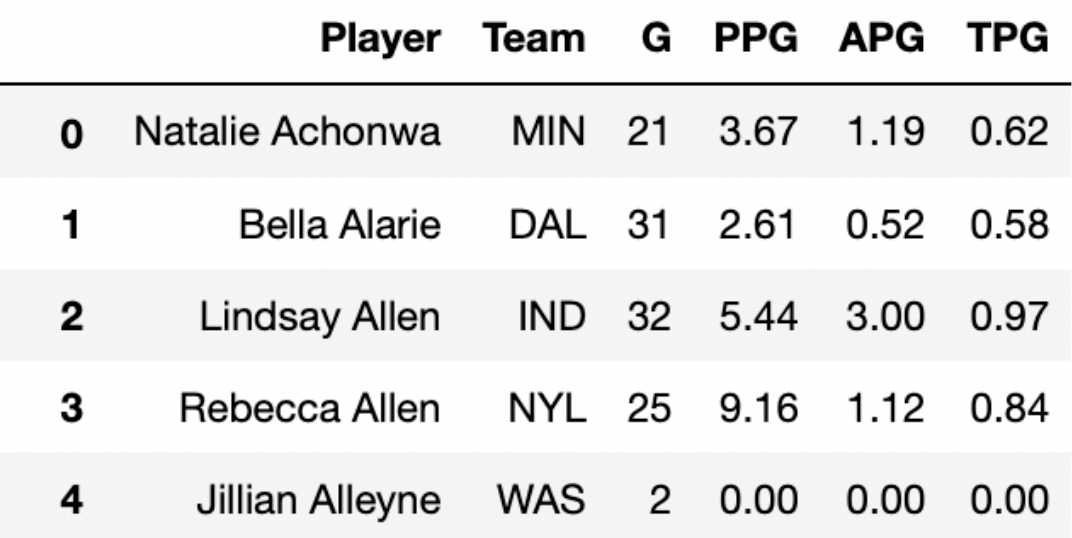
Given below is the season DataFrame, which contains
statistics on all players in the WNBA in the 2021 season. The first few
rows of season are shown below:
Each row in season corresponds to a single player. In this problem,
we’ll be looking at the 'PPG' column, which records the
number of points scored per game played.
Now, suppose we only have access to the DataFrame
small_season, which is a random sample of size
36 from season. We’re interested in learning about
the true mean points per game of all players in season
given just the information in small_season.
To start, we want to bootstrap small_season 10,000 times
and compute the mean of the resample each time. We want to store these
10,000 bootstrapped means in the array boot_means.
Here is a broken implementation of this procedure.
boot_means = np.array([])
for i in np.arange(10000):
    resample = small_season.sample(season.shape[0], replace=False)  # Line 1
    resample_mean = small_season.get('PPG').mean()                  # Line 2
    np.append(boot_means, new_mean)                                 # Line 3
For each of the 3 lines of code above (marked by comments), specify what is incorrect about the line by selecting one or more of the corresponding options below. Or, select “Line _ is correct as-is” if you believe there’s nothing that needs to be changed about the line in order for the above code to run properly.
What is incorrect about Line 1? Select all that apply.
Currently the procedure samples from small_season, when
it should be sampling from season
The sample size is season.shape[0], when it should be
small_season.shape[0]
Sampling is currently being done without replacement, when it should be done with replacement
Line 1 is correct as-is
Answers:
season.shape[0], when it should be
small_season.shape[0]Here, our goal is to bootstrap from small_season. When
bootstrapping, we sample with replacement from our
original sample, with a sample size that’s equal to the original
sample’s size. Here, our original sample is small_season,
so we should be taking samples of size
small_season.shape[0] from it.
Option 1 is incorrect; season has nothing to do with
this problem, as we are bootstrapping from
small_season.
The average score on this problem was 95%.
What is incorrect about Line 2? Select all that apply.
Currently it is taking the mean of the 'PPG' column in
small_season, when it should be taking the mean of the
'PPG' column in season
Currently it is taking the mean of the 'PPG' column in
small_season, when it should be taking the mean of the
'PPG' column in resample
.mean() is not a valid Series method, and should be
replaced with a call to the function np.mean
Line 2 is correct as-is
Answer: Currently it is taking the mean of the
'PPG' column in small_season, when it should
be taking the mean of the 'PPG' column in
resample
The current implementation of Line 2 doesn’t use the
resample at all, when it should. If we were to leave Line 2
as it is, all of the values in boot_means would be
identical (and equal to the mean of the 'PPG' column in
small_season).
Option 1 is incorrect since our bootstrapping procedure is
independent of season. Option 3 is incorrect because
.mean() is a valid Series method.
The average score on this problem was 98%.
What is incorrect about Line 3? Select all that apply.
The result of calling np.append is not being reassigned
to boot_means, so boot_means will be an empty
array after running this procedure
The indentation level of the line is incorrect –
np.append should be outside of the for-loop
(and aligned with for i)
new_mean is not a defined variable name, and should be
replaced with resample_mean
Line 3 is correct as-is
Answers:
np.append is not being reassigned
to boot_means, so boot_means will be an empty
array after running this procedurenew_mean is not a defined variable name, and should be
replaced with resample_meannp.append returns a new array and does not modify the
array it is called on (boot_means, in this case), so Option
1 is a necessary fix. Furthermore, Option 3 is a necessary fix since
new_mean wasn’t defined anywhere.
Option 2 is incorrect; if np.append were outside of the
for-loop, none of the 10,000 resampled means would be saved
in boot_means.
The average score on this problem was 94%.
We construct a 95% confidence interval for the true mean points per game for all players by taking the middle 95% of the bootstrapped sample means.
left_b = np.percentile(boot_means, 2.5)
right_b = np.percentile(boot_means, 97.5)
boot_ci = [left_b, right_b]
We find that boot_ci is the interval [7.7, 10.3].
However, the mean points per game in season is 7, which is
not in the interval we found. Which of the following statements is true?
(Select all that apply)
95% of games in season have a number of points between
7.7 and 10.3.
95% of values in boot_means fall between 7.7 and
10.3.
There is a 95% chance that the true mean points per game is between 7.7 and 10.3.
The interval we created did not contain the true mean points per game, but if we collected many original samples and constructed many 95% confidence intervals, then exactly 95% of them would contain the true mean points per game.
The interval we created did not contain the true mean points per game, but if we collected many original samples and constructed many 95% confidence intervals, then roughly 95% of them would contain the true mean points per game.
Answers:
boot_means fall between the endpoints
of the interval we found.The first option is incorrect because the confidence interval describes what we think the mean points per game could be. Individual games likely have a very large variety in the number of points scored. Probably very few have between 7.7 and 10.3 points.
The second option is correct because this is precisely how we
calculated the endpoints of our interval, by taking the middle 95% of
values in boot_means.
The third option is incorrect because we know the true mean points per game - it’s 7. 7 does not fall in the interval 7.7 to 10.3, and we can say that with certainty. This is not a probability statement because the interval and the parameter are both fixed.
The fourth option is incorrect because of the word exactly. We generally can’t make guarantees like this when working with randomness.
The fifth option is correct, as this is the meaning of confidence. We have confidence in the process of generating 95% confidence intervals, because roughly 95% of such intervals we create will capture the parameter of interest.
True or False: Suppose that from a sample, you compute a 95% bootstrapped confidence interval for a population parameter to be the interval [L, R]. Then the average of L and R is the mean of the original sample.
Answer: False
A 95% confidence interval indicates we are 95% confident that the true population parameter falls within the interval [L, R]. Note that the problem specifies that the confidence interval is bootstrapped. Since the interval is found using bootstrapping, L and R averaged will not be the mean of the original sample since the mean of the original sample is not what is used in calculating the bootstrapped confidence interval. The bootstrapped confidence interval is created by re-sampling the data with replacement over and over again. Thus, while the interval is typically centered around the sample mean due to the nature of bootstrapping, the average of L and R (the 2.5th and 97.5th percentiles of the distribution of bootstrapped means) may not exactly equal the sample mean, but should be close to it. Additionally, L is the 2.5th percentile of the distribution of bootstrapped means and R is the 97.5th percentile, and these are not necessarily the same distance away from the mean of the sample.
The average score on this problem was 87%.
results = np.array([])
for i in np.arange(10):
    result = np.random.choice(np.arange(1000), replace=False)
    results = np.append(results, result)
After this code executes, results contains:
a simple random sample of size 9, chosen from a set of size 999 with replacement
a simple random sample of size 9, chosen from a set of size 999 without replacement
a simple random sample of size 10, chosen from a set of size 1000 with replacement
a simple random sample of size 10, chosen from a set of size 1000 without replacement
Answer: a simple random sample of size 10, chosen from a set of size 1000 with replacement
Let’s see what the code is doing. The first line initializes an empty
array called results. The for loop runs 10 times. Each
time, it creates a value called result by some process
we’ll inspect shortly and appends this value to the end of the
results array. At the end of the code snippet,
results will be an array containing 10 elements.
Now, let’s look at the process by which each element
result is generated. Each result is a random
element chosen from np.arange(1000) which is the numbers
from 0 to 999, inclusive. That’s 1000 possible numbers. Each time
np.random.choice is called, just one value is chosen from
this set of 1000 possible numbers.
When we sample just one element from a set of values, sampling with replacement is the same as sampling without replacement, because sampling with or without replacement concerns whether subsequent draws can be the same as previous ones. When we’re just sampling one element, it really doesn’t matter whether our process involves putting that element back, as we’re not going to draw again!
Therefore, result is just one random number chosen from
the 1000 possible numbers. Each time the for loop executes,
result gets set to a random number chosen from the 1000
possible numbers. It is possible (though unlikely) that the random
result of the first execution of the loop matches the
result of the second execution of the loop. More generally,
there can be repeated values in the results array since
each entry of this array is independently drawn from the same set of
possibilities. Since repetitions are possible, this means the sample is
drawn with replacement.
Therefore, the results array contains a sample of size
10 chosen from a set of size 1000 with replacement. This is called a
“simple random sample” because each possible sample of 10 values is
equally likely, which comes from the fact that
np.random.choice chooses each possible value with equal
probability by default.
The average score on this problem was 11%.
An IKEA fan created an app where people can log the amount of time it
took them to assemble their IKEA furniture. The DataFrame
app_data has a row for each product build that was logged
on the app. The columns are:
'product' (str): the name of the product,
which includes the product line as the first word, followed by a
description of the product'category' (str): a categorical
description of the type of product'assembly_time' (str): the amount of time
to assemble the product, formatted as 'x hr, y min' where
x and y represent integers, possibly zero'minutes' (int): integer values
representing the number of minutes it took to assemble each product
We want to use app_data to estimate the average amount
of time it takes to build an IKEA bed (any product in the
'bed' category). Which of the following strategies would be
an appropriate way to estimate this quantity? Select all that apply.
Query to keep only the beds. Then resample with replacement many
times. For each resample, take the mean of the 'minutes'
column. Compute a 95% confidence interval based on those means.
Query to keep only the beds. Group by 'product' using
the mean aggregation function. Then resample with replacement many
times. For each resample, take the mean of the 'minutes'
column. Compute a 95% confidence interval based on those means.
Resample with replacement many times. For each resample, first query
to keep only the beds and then take the mean of the
'minutes' column. Compute a 95% confidence interval based
on those means.
Resample with replacement many times. For each resample, first query
to keep only the beds. Then group by 'product' using the
mean aggregation function, and finally take the mean of the
'minutes' column. Compute a 95% confidence interval based
on those means.
Answer: Option 1
Only the first answer is correct. This is a question of parameter estimation, so our approach is to use bootstrapping to create many resamples of our original sample, computing the average of each resample. Each resample should always be the same size as the original sample. The first answer choice accomplishes this by querying first to keep only the beds, then resampling from the DataFrame of beds only. This means resamples will have the same size as the original sample. Each resample’s mean will be computed, so we will have many resample means from which to construct our 95% confidence interval.
In the second answer choice, we are actually taking the mean twice.
We first average the build times for all builds of the same product when
grouping by product. This produces a DataFrame of different products
with the average build time for each. We then resample from this
DataFrame, computing the average of each resample. But this is a
resample of products, not of product builds. The size of the resample is
the number of unique products in app_data, not the number
of reported product builds in app_data. Further, we get
incorrect results by averaging numbers that are already averages. For
example, if 5 people build bed A and it takes them each 1 hour, and 1
person builds bed B and it takes them 10 hours, the average amount of
time to build a bed is \frac{5*1+10}{6} =
2.5. But if we average the times for bed A (1 hour) and average
the times for bed B (5 hours), then average those, we get \frac{1+5}{2} = 3, which is not the same.
More generally, grouping is not a part of the bootstrapping process
because we want each data value to be weighted equally.
The last two answer choices are incorrect because they involve
resampling from the full app_data DataFrame before querying
to keep only the beds. This is incorrect because it does not preserve
the sample size. For example, if app_data contains 1000
reported bed builds and 4000 other product builds, then the only
relevant data is the 1000 bed build times, so when we resample, we want
to consider another set of 1000 beds. If we resample from the full
app_data DataFrame, our resample will contain 5000 rows,
but the number of beds will be random, not necessarily 1000. If we query
first to keep only the beds, then resample, our resample will contain
exactly 1000 beds every time. As an added bonus, since we only care
about beds, it’s much faster to resample from a smaller DataFrame of
beds only than it is to resample from all app_data with
plenty of rows we don’t care about.
The average score on this problem was 71%.
Suppose we have access to a simple random sample of all US Costco
members of size 145. Our sample is stored in a
DataFrame named us_sample, in which the
"Spend" column contains the October 2023 spending of each
sampled member in dollars.
Fill in the blanks below so that us_left and
us_right are the left and right endpoints of a
46% confidence interval for the average October 2023
spending of all US members.
costco_means = np.array([])
for i in np.arange(5000):
    resampled_spends = __(x)__
    costco_means = np.append(costco_means, resampled_spends.mean())
us_left = np.percentile(costco_means, __(y)__)
us_right = np.percentile(costco_means, __(z)__)
Which of the following could go in blank (x)? Select all that apply.
us_sample.sample(145, replace=True).get("Spend")
us_sample.sample(145, replace=False).get("Spend")
np.random.choice(us_sample.get("Spend"), 145)
np.random.choice(us_sample.get("Spend"), 145, replace=True)
np.random.choice(us_sample.get("Spend"), 145, replace=False)
None of the above.
What goes in blanks (y) and (z)? Give your answers as integers.
Answer:
x:
us_sample.sample(145, replace=True).get("Spend")np.random.choice(us_sample.get("Spend"), 145)np.random.choice(us_sample.get("Spend"), 145, replace=True)y: 27z: 73
The average score on this problem was 79%.
True or False: 46% of all US members in
us_sample spent between us_left and
us_right in October 2023.
True
False
Answer: False
The average score on this problem was 85%.
True or False: If we repeat the code from part (b) 200 times, each time bootstrapping from a new random sample of 145 members drawn from all US members, then about 92 of the intervals we create will contain the average October 2023 spending of all US members.
True
False
Answer: True
The average score on this problem was 51%.
True or False: If we repeat the code from part (b) 200 times, each
time bootstrapping from us_sample, then about
92 of the intervals we create will contain the average
October 2023 spending of all US members.
True
False
Answer: False
The average score on this problem was 30%.
The Oscars, or Academy Awards, are the highest awards in the film
industry, awarded each year to the best movies of that year. The
oscars DataFrame contains a row for each movie that has
ever been nominated for an Oscar. The "name" column
contains the name of the movie and the "rating" column
contains a rating of the movie on a 0 to 100 scale. This number
incorporates many factors, but we won’t worry about how it is
computed.

Fill in the blanks below to collect a simple random
sample of 400 movies from the oscars DataFrame,
then calculate 10,000 bootstrapped sample mean ratings.
my_sample = __(x)__
n_resamples = 10000
boot_means = np.array([])
for i in np.arange(n_resamples):
    resample = __(y)__
    mean = __(z)__
boot_means = np.append(boot_means, mean)Answer (x): oscars.sample(400)
The average score on this problem was 85%.
Answer (y):
my_sample.sample(400, replace=True)
The average score on this problem was 87%.
Answer (z):
resample.get("rating").mean()
The average score on this problem was 96%.
In each blank, circle the word that correctly fills in the
sentence.
A histogram of boot_means shows a(n)
probability / empirical distribution
of a statistic / parameter.
Answer: empirical, statistic
The average score on this problem was 77%.
Suppose we use the array boot_means to calculate a 90%
confidence interval for the mean rating of Oscar-nominated movies.
Select all correct conclusions we can draw about this
interval.
There is a 90% chance that the true mean rating of all Oscar-nominated movies falls within this interval.
The sample mean rating is within 90% of the true mean rating of all Oscar-nominated movies.
If we looked at the ratings of many Oscar-nominated movies, about 90% of them would fall within this range.
None of the above.
Answer: None of the above.
The average score on this problem was 74%.
The DataFrame restaurants contains information about a
sample of restaurants in San Diego County. We have each restaurant’s
"name" (str), "rating" (int), average
"meal_price" (float), and type of
"cuisine" (str), such as "Thai" or
"Italian".
You are interested in estimating the average
"meal_price" across all Italian restaurants in San Diego
County using only the data in restaurants. Fill in the
following code so that italian_means evaluates to an array
of 1000 bootstrapped estimates for this parameter.
    def bootstrap_means(data, n_samples):
        means = np.array([])
        for i in range(n_samples):
            resample = data.sample(__(a)__, replace = __(b)__)
            means = np.append(means, __(c)__)
        return means

    italian_restaurants = __(d)__
italian_means = bootstrap_means(italian_restaurants, __(e)__)(a): data.shape[0]
(b): True
(c): resample.get("meal_price").mean()
(d):
restaurants[restaurants.get("cuisine") == "Italian"]
(e): 1000
The average score on this problem was 73%.
Next, fill in the blanks below so that italian_CI
evaluates to an 88% bootstrapped confidence interval for the average
"meal_price" across all Italian restaurants in San Diego
County.
    lower_bound = np.percentile(italian_means, __(a)__)
    upper_bound = np.percentile(italian_means, __(b)__)
italian_CI = [lower_bound, upper_bound](a): 6
(b): 94
The average score on this problem was 83%.
Suppose italian_CI evaluates to [25, 35]. Which of the
following statements are correct? Select all that apply.
If we randomly selected 1000 Italian restaurants from the population
of Italian restaurants in San Diego County, about 880 of them will have
an average "meal_price" between $25 and $35.
There is an 88% chance that the average "meal_price" of
Italian restaurants in San Diego County falls between $25 and $35.
88% of all Italian restaurants have an average
"meal_price" between $25 and $35.
None of the above.
Option 4: None of the above.
The average score on this problem was 64%.
Which of the following can be used to generate a simple
random sample of "rating"s from 10 restaurants in
restaurants? Select all that apply.
Option 1:
sample = restaurants.take(np.arange(10)).get("rating")Option 2:
sample = restaurants.sample(10, replace = False).get("rating")Option 3:
sample = restaurants.sample(10, replace = True).get("rating")Option 4:
    positions = np.random.choice(np.arange(0, restaurants.shape[0]),
                                 10, replace = False)
    sample = restaurants.take(positions).get("rating")
Option 5:
    positions = np.random.choice(np.arange(0, restaurants.shape[0]),
                                 10, replace = True)
    sample = restaurants.take(positions).get("rating")
Option 1
Option 2
Option 3
Option 4
Option 5
Options 2 and 4
The average score on this problem was 65%.