← return to practice.dsc10.com
These problems are taken from past quizzes and exams. Work on them
on paper, since the quizzes and exams you take in this
course will also be on paper.
We encourage you to complete these
problems during discussion section. Solutions will be made available
after all discussion sections have concluded. You don’t need to submit
your answers anywhere.
Note: We do not plan to cover all of
these problems during the discussion section; the problems we don’t
cover can be used for extra practice.
Rank these three students in ascending order of their exam performance relative to their classmates.
Hector, Clara, Vivek
Vivek, Hector, Clara
Clara, Hector, Vivek
Vivek, Clara, Hector
Answer: Vivek, Hector, Clara
To compare Vivek, Hector, and Clara’s relative performance we want to compare their Z scores to handle standardization. For Vivek, his Z score is (83-75) / 6 = 4/3. For Hector, his score is (77-70) / 5 = 7/5. For Clara, her score is (80-75) / 3 = 5/3. Ranking these, 5/3 > 7/5 > 4/3 which yields the result of Vivek, Hector, Clara.
The average score on this problem was 76%.
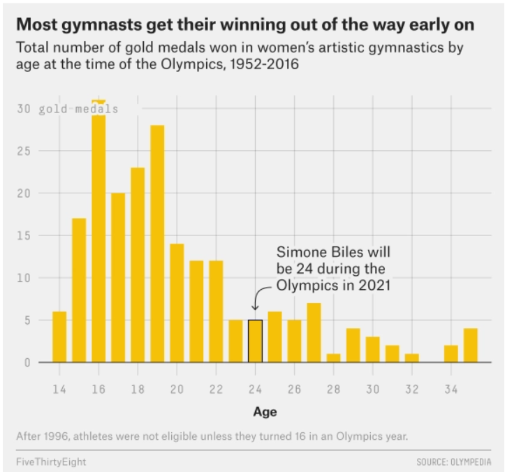
The data visualization below shows all Olympic gold medals for women’s gymnastics, broken down by the age of the gymnast.
Based on this data, rank the following three quantities in ascending order: the median age at which gold medals are earned, the mean age at which gold medals are earned, the standard deviation of the age at which gold medals are earned.
mean, median, SD
median, mean, SD
SD, mean, median
SD, median, mean
Answer: SD, median, mean
The standard deviation will clearly be the smallest of the three
values as most of the data is encompassed between the range of
[14-26]. Intuitively, the standard deviation will have to
be about a third of this range which is around 4 (though this is not the
exact standard deviation, but is clearly much less than the mean and
median with values closer to 19-25). Comparing the median and mean, it
is important to visualize that this distribution is skewed right. When
the data is skewed right it pulls the mean towards a higher value (as
the higher values naturally make the average higher). Therefore, we know
that the mean will be greater than the median and the ranking is SD,
median, mean.
The average score on this problem was 72%.
Among all Costco members in San Diego, the average monthly spending in October 2023 was $350 with a standard deviation of $40.
The amount Ciro spent at Costco in October 2023 was -1.5 in standard units. What is this amount in dollars? Give your answer as an integer.
Answer: 290
The average score on this problem was 93%.
What is the minimum possible percentage of San Diego members that spent between $250 and $450 in October 2023?
16%
22%
36%
60%
78%
84%
Answer: 84%
The average score on this problem was 61%.
Now, suppose we’re given that the distribution of monthly spending in October 2023 for all San Diego members is roughly normal. Given this fact, fill in the blanks:
What are m and n? Give your answers as integers rounded to the nearest multiple of 10.
Answer: m: 270, n: 430
The average score on this problem was 81%.
Researchers from the San Diego Zoo, located within Balboa Park, collected physical measurements of several species of penguins in a region of Antarctica.
One piece of information they tracked for each of 330 penguins was its mass in grams. The average penguin mass is 4200 grams, and the standard deviation is 840 grams.
Consider the histogram of mass below.
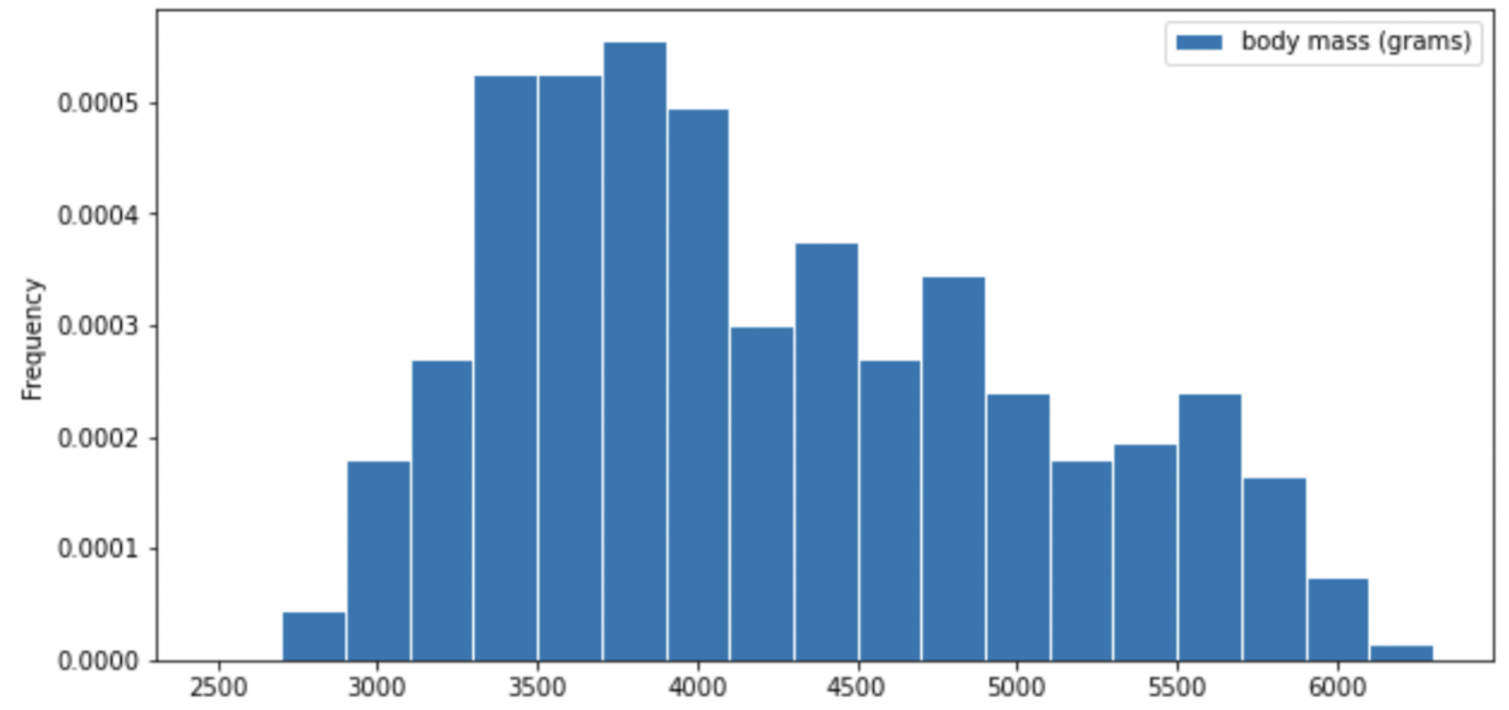
Select the true statement below.
The median mass of penguins is larger than the average mass of penguins
The median mass of penguins is roughly equal to the average mass of penguins (within 50 grams)
The median mass of penguins is less than the average mass of penguins
It is impossible to determine the relationship between the median and average mass of penguins just by looking at the above histogram
Answer: The median mass of penguins is less than the average mass of penguins
This is a distribution that is skewed to the right, so mean is greater than median.
The average score on this problem was 87%.
For your convenience, we show the histogram of mass again below.
Recall, there are 330 penguins in our dataset. Their average mass is 4200 grams, and the standard deviation of mass is 840 grams.
Per Chebyshev’s inequality, at least what percentage of penguins have a mass between 3276 grams and 5124 grams? Input your answer as a percentage between 0 and 100, without the % symbol. Round to three decimal places.
Answer: 17.355
Recall, Chebyshev’s inequality states that No matter what the shape of the distribution is, the proportion of values in the range “average ± z SDs” is at least 1 - \frac{1}{z^2}.
To approach the problem, we’ll start by converting 3276 grams and 5124 grams to standard units. Doing so yields \frac{3276 - 4200}{840} = -1.1, similarly, \frac{5124 - 4200}{840} = 1.1. This means that 3276 is 1.1 standard deviations below the mean, and 5124 is 1.1 standard deviations above the mean. Thus, we are calculating the proportion of values in the range “average ± 1.1 SDs”.
When z = 1.1, we have 1 - \frac{1}{z^2} = 1 - \frac{1}{1.1^2} \approx 0.173553719, which as a percentage rounded to three decimal places is 17.355\%.
The average score on this problem was 76%.
Per Chebyshev’s inequality, at least what percentage of penguins have a mass between 1680 grams and 5880 grams?
50%
55.5%
65.25%
68%
75%
88.8%
95%
Answer: 75%
Recall: proportion with z SDs of the mean
| Percent in Range | All Distributions (via Chebyshev’s Inequality) | Normal Distributions |
|---|---|---|
| \text{average} \pm 1 \ \text{SD} | \geq 0\% | \approx 68\% |
| \text{average} \pm 2\text{SDs} | \geq 75\% | \approx 95\% |
| \text{average} \pm 3\text{SDs} | \geq 88\% | \approx 99.73\% |
To approach the problem, we’ll start by converting 3276 grams and 5124 grams to standard units. Doing so yields \frac{1680 - 4200}{840} = -3, similarly, \frac{5880 - 4200}{840} = 2. This means that 1680 is 3 standard deviations below the mean, and 5880 is 2 standard deviations above the mean.
Proportion of values in [-3 SUs, 2 SUs] >= Proportion of values in [-2 SUs, 2 SUs] >= 75% (Since we cannot assume that the distribution is normal, we look at the All Distributions (via Chebyshev’s Inequality) column for proportion).
Thus, at least 75% of the penguins have a mass between 1680 grams and 5880 grams.
The average score on this problem was 72%.
The distribution of mass in grams is not roughly normal. Is the distribution of mass in standard units roughly normal?
Yes
No
Impossible to tell
Answer: No
The shape of the distribution does not change since we are scaling the x values for all data.
The average score on this problem was 60%.
Suppose boot_means is an array of the resampled means.
Fill in the blanks below so that [left, right] is a 68%
confidence interval for the true mean mass of penguins.
left = np.percentile(boot_means, __(a)__)
right = np.percentile(boot_means, __(b)__)
[left, right]
What goes in blank (a)? What goes in blank (b)?
Answer: (a) 16 (b) 84
Recall, np.percentile(array, p) computes the
pth percentile of the numbers in array. To
compute the 68% CI, we need to know the percentile of left tail and
right tail.
left percentile = (1-0.68)/2 = (0.32)/2 = 0.16 so we have 16th percentile
right percentile = 1-((1-0.68)/2) = 1-((0.32)/2) = 1-0.16 = 0.84 so we have 84th percentile
The average score on this problem was 94%.
Which of the following is a correct interpretation of this confidence interval? Select all that apply.
There is an approximately 68% chance that mean weight of all penguins in Antarctica falls within the bounds of this confidence interval.
Approximately 68% of penguin weights in our sample fall within the bounds of this confidence interval.
Approximately 68% of penguin weights in the population fall within the bounds of this interval.
If we created many confidence intervals using the same method, approximately 68% of them would contain the mean weight of all penguins in Antarctica.
None of the above
Answer: Option 4 (If we created many confidence intervals using the same method, approximately 68% of them would contain the mean weight of all penguins in Antarctica.)
Recall, what a k% confidence level states is that approximately k% of the time, the intervals you create through this process will contain the true population parameter.
In this question, our population parameter is the mean weight of all penguins in Antarctica. So 86% of the time, the intervals you create through this process will contain the mean weight of all penguins in Antarctica. This is the same as Option 4. However, it will be false if we state it in the reverse order (Option 1) since our population parameter is already fixed.
The average score on this problem was 81%.
An IKEA chair designer is experimenting with some new ideas for armchair designs. She has the idea of making the arm rests shaped like bell curves, or normal distributions. A cross-section of the armchair design is shown below.
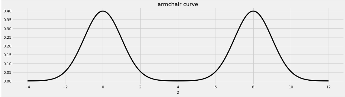
This was created by taking the portion of the standard normal distribution from z=-4 to z=4 and adjoining two copies of it, one centered at z=0 and the other centered at z=8. Let’s call this shape the armchair curve.
Since the area under the standard normal curve from z=-4 to z=4 is approximately 1, the total area under the armchair curve is approximately 2.
Complete the implementation of the two functions below:
area_left_of(z) should return the area under the
armchair curve to the left of z, assuming
-4 <= z <= 12, andarea_between(x, y) should return the area under the
armchair curve between x and y, assuming
-4 <= x <= y <= 12.import scipy
def area_left_of(z):
'''Returns the area under the armchair curve to the left of z.
Assume -4 <= z <= 12'''
if ___(a)___:
return ___(b)___
return scipy.stats.norm.cdf(z)
def area_between(x, y):
'''Returns the area under the armchair curve between x and y.
Assume -4 <= x <= y <= 12.'''
return ___(c)___What goes in blank (a)?
Answer: z>4 or
z>=4
The body of the function contains an if statement
followed by a return statement, which executes only when
the if condition is false. In that case, the function
returns scipy.stats.norm.cdf(z), which is the area under
the standard normal curve to the left of z. When
z is in the left half of the armchair curve, the area under
the armchair curve to the left of z is the area under the
standard normal curve to the left of z because the left
half of the armchair curve is a standard normal curve, centered at 0. So
we want to execute the return statement in that case, but
not if z is in the right half of the armchair curve, since
in that case the area to the left of z under the armchair
curve should be more than 1, and scipy.stats.norm.cdf(z)
can never exceed 1. This means the if condition needs to
correspond to z being in the right half of the armchair
curve, which corresponds to z>4 or z>=4,
either of which is a correct solution.
The average score on this problem was 72%.
What goes in blank (b)?
Answer:
1+scipy.stats.norm.cdf(z-8)
This blank should contain the value we want to return when
z is in the right half of the armchair curve. In this case,
the area under the armchair curve to the left of z is the
sum of two areas:
z.Since the right half of the armchair curve is just a standard normal
curve that’s been shifted to the right by 8 units, the area under that
normal curve to the left of z is the same as the area to
the left of z-8 on the standard normal curve that’s
centered at 0. Adding the portion from the left half and the right half
of the armchair curve gives
1+scipy.stats.norm.cdf(z-8).
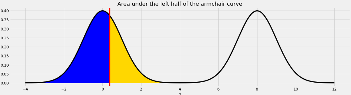
For example, if we want to find the area under the armchair curve to the left of 9, we need to total the yellow and blue areas in the image below.
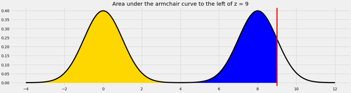
The yellow area is 1 and the blue area is the same as the area under the standard normal curve (or the left half of the armchair curve) to the left of 1 because 1 is the point on the left half of the armchair curve that corresponds to 9 on the right half. In general, we need to subtract 8 from a value on the right half to get the corresponding value on the left half.
The average score on this problem was 54%.
What goes in blank (c)?
Answer:
area_left_of(y) - area_left_of(x)
In general, we can find the area under any curve between
x and y by taking the area under the curve to
the left of y and subtracting the area under the curve to
the left of x. Since we have a function to find the area to
the left of any given point in the armchair curve, we just need to call
that function twice with the appropriate inputs and subtract the
result.
The average score on this problem was 60%.
Suppose you have correctly implemented the function
area_between(x, y) so that it returns the area under the
armchair curve between x and y, assuming the
inputs satisfy -4 <= x <= y <= 12.
Note: You can still do this question, even if you didn’t know how to do the previous one.
What is the approximate value of
area_between(-2, 10)?
1.9
1.95
1.975
2
Answer: 1.95
The area we want to find is shown below in two colors. We can find the area in each half of the armchair curve separately and add the results.
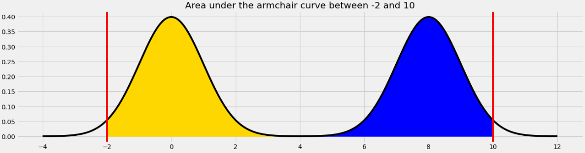
For the yellow area, we know that the area within 2 standard deviations of the mean on the standard normal curve is 0.95. The remaining 0.05 is split equally on both sides, so the yellow area is 0.975.
The blue area is the same by symmetry so the total shaded area is 0.975*2 = 1.95.
Equivalently, we can use the fact that the total area under the armchair curve is 2, and the amount of unshaded area on either side is 0.025, so the total shaded area is 2 - (0.025*2) = 1.95.
The average score on this problem was 76%.
What is the approximate value of
area_between(0.37, 8.37)?
0.68
0.95
1
1.5
Answer: 1
The area we want to find is shown below in two colors.
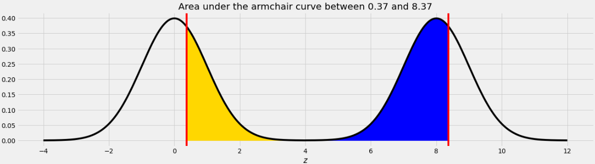
As we saw in Problem 12.2, the point on the left half of the armchair curve that corresponds to 8.37 is 0.37. This means that if we move the blue area from the right half of the armchair curve to the left half, it will fit perfectly, as shown below.
Therefore the total of the blue and yellow areas is the same as the area under one standard normal curve, which is 1.
The average score on this problem was 76%.
Beneath Gringotts Wizarding Bank, enchanted mine carts transport wizards through a complex underground railway on the way to their bank vault.
During one section of the journey to Harry’s vault, the track follows the shape of a normal curve, with a peak at x = 50 and a standard deviation of 20.
A ferocious dragon, who lives under this section of the railway, is equally likely to be located anywhere within this region. What is the probability that the dragon is located in a position with x \leq 10 or x \geq 80? Select all that apply.
1 - (scipy.stats.norm.cdf(1.5) - scipy.stats.norm.cdf(-2))
2 * scipy.stats.norm.cdf(1.75)
scipy.stats.norm.cdf(-2) + scipy.stats.norm.cdf(-1.5)
0.95
None of the above.
Answer:
1 - (scipy.stats.norm.cdf(1.5) - scipy.stats.norm.cdf(-2))
&
scipy.stats.norm.cdf(-2) + scipy.stats.norm.cdf(-1.5)
Option 1: This code calculates the probability that a value lies outside the range between z = -2 and z = 1.5, which corresponds to x \leq 10 or x \geq 80. This is done by subtracting the area under the normal curve between -2 and 1.5 from 1. This is correct because it accurately captures the combined probability in the left and right tails of the distribution.
Option 2: This code multiplies the cumulative distribution function (CDF) at z = 1.75 by 2. This assumes symmetry around the mean and is used for intervals like |z| \geq 1.75, but that’s not what we want. The correct z-values for this problem are -2 and 1.5, so this option is incorrect.
Option 3: This code adds the probability of z \leq -2 and z \geq 1.5, using the fact that P(z \geq 1.5) = P(z \leq -1.5) by symmetry. So, while the code appears to show both as left-tail calculations, it actually produces the correct total tail probability. This option is correct.
Option 4: This is a static value with no basis in the z-scores of -2 and 1.5. It’s likely meant as a distractor and does not represent the correct probability for the specified conditions. This option is incorrect.
Harry wants to know where, in this section of the track, the cart’s height is changing the fastest. He knows from his earlier public school education that the height changes the fastest at the inflection points of a normal distribution. Where are the inflection points in this section of the track?
x = 50
x = 20 and x = 80
x = 30 and x = 70
x = 0 and x = 100
Answer: x = 30 and x = 70
Recall that the inflection points of a normal distribution are located one standard deviation away from the mean. In this problem, the mean is x = 50 and the standard deviation is 20, so the inflection points occur at x = 30 and x = 70. These are the points where the curve changes concavity and where the height is changing the fastest. Therefore, the correct answer is x = 30 and x = 70.
Next, consider a different region of the track, where the shape follows some arbitrary distribution with mean 130 and standard deviation 30. We don’t have any information about the shape of the distribution, so it is not necessarily normal.
What is the minimum proportion of area under this section of the track within the range 100 \leq x \leq 190?
0.77
0.55
0.38
0.00
Answer: 0.00
We are told that the distribution is not necessarily normal. The mean is 130 and the standard deviation is 30. We’re asked for the minimum proportion of area between x = 100 and x = 190.
Since the distribution isn’t normal and we don’t know its shape, we can’t use the empirical rule (68-95-99.7) or z-scores. We might try using Chebyshev’s Inequality, but that only works for intervals that are equally far below the mean as above the mean. This interval is not like that (it’s 1 standard deviation below the mean and 2 above), so Chebyshev’s Inequality doesn’t apply. The most we can say using Chebyshev’s Inequality is that in the interval from 1 standard deviation below the mean to 1 standard deviation above the mean, we can get at least 1 - \frac{1}{0^2} = 0 percent of the data. We can’t make any additional guarantees. So, the minimum possible proportion of area is 0.00.