These problems are taken from past quizzes and exams. Work on them
on paper, since the quizzes and exams you take in this
course will also be on paper.
We encourage you to complete these
problems during discussion section. Solutions will be made available
after all discussion sections have concluded. You don’t need to submit
your answers anywhere.
Note: We do not plan to cover all of
these problems during the discussion section; the problems we don’t
cover can be used for extra practice.
Problem 1
Lecture
17
Oren has a random sample of 200 dog prices in an array called
oren. He has also bootstrapped his sample 1,000 times and
stored the mean of each resample in an array called
boots.
In this question, assume that the following code has run:
a = np.mean(oren)b = np.std(oren)c =len(oren)
Problem 1.1
What expression best estimates the population’s standard
deviation?
b
b / c
b / np.sqrt(c)
b * np.sqrt(c)
Answer: b
The function np.std directly calculated the standard
deviation of array oren. Even though oren is
sample of the population, its standard deviation is still a pretty good
estimate for the standard deviation of the population because it is a
random sample. The other options don’t really make sense in this
context.
Difficulty: ⭐️⭐️⭐️
The average score on this problem was 57%.
Problem 1.2
Which expression best estimates the mean of boots?
0
a
(oren - a).mean()
(oren - a) / b
Answer: a
Note that a is equal to the mean of oren,
which is a pretty good estimator of the mean of the overall population
as well as the mean of the distribution of sample means. The other
options don’t really make sense in this context.
Difficulty: ⭐️⭐️
The average score on this problem was 89%.
Problem 1.3
What expression best estimates the standard deviation of
boots?
b
b / c
b / np.sqrt(c)
(a -b) / np.sqrt(c)
Answer: b / np.sqrt(c)
Note that we can use the Central Limit Theorem for this problem which
states that the standard deviation (SD) of the distribution of sample
means is equal to (population SD) / np.sqrt(sample size).
Since the SD of the sample is also the SD of the population in this
case, we can plug our variables in to see that
b / np.sqrt(c) is the answer.
Difficulty: ⭐️
The average score on this problem was 91%.
Problem 1.4
What is the dog price of $560 in standard units?
(560 - a) / b
(560 - a) / (b / np.sqrt(c))
(a - 560) / (b / np.sqrt(c))}
abs(560 - a) / b
abs(560 - a) / (b / np.sqrt(c))
Answer: (560 - a) / b
To convert a value to standard units, we take the value, subtract the
mean from it, and divide by SD. In this case that is
(560 - a) / b, because a is the mean of our
dog prices sample array and b is the SD of the dog prices
sample array.
Difficulty: ⭐️⭐️
The average score on this problem was 80%.
Problem 1.5
The distribution of boots is normal because of the
Central Limit Theorem.
True
False
Answer: True
True. The central limit theorem states that if you have a population
and you take a sufficiently large number of random samples from the
population, then the distribution of the sample means will be
approximately normally distributed.
Difficulty: ⭐️
The average score on this problem was 91%.
Problem 1.6
If Oren’s sample was 400 dogs instead of 200, the standard deviation
of boots will…
Increase by a factor of 2
Increase by a factor of \sqrt{2}
Decrease by a factor of 2
Decrease by a factor of \sqrt{2}
None of the above
Answer: Decrease by a factor of \sqrt{2}
Recall that the central limit theorem states that the STD of the
sample distribution is equal to
(population STD) / np.sqrt(sample size). So if we increase
the sample size by a factor of 2, the STD of the sample distribution
will decrease by a factor of \sqrt{2}.
Difficulty: ⭐️⭐️
The average score on this problem was 80%.
Problem 1.7
If Oren took 4000 bootstrap resamples instead of 1000, the standard
deviation of boots will…
Increase by a factor of 4
Increase by a factor of 2
Decrease by a factor of 2
Decrease by a factor of 4
None of the above
Answer: None of the above
Again, from our formula given by the central limit theorem, the
sample STD doesn’t depend on the number of bootstrap resamples so long
as it’s “sufficiently large”. Thus increasing our bootstrap sample from
1000 to 4000 will have no effect on the std of boots
Difficulty: ⭐️⭐️⭐️
The average score on this problem was 74%.
Problem 1.8
Write one line of code that evaluates to the right
endpoint of a 92% CLT-Based confidence interval for the mean
dog price. The following expressions may help:
Recall that a 92% confidence interval means an interval that consists
of the middle 92% of the distribution. In other words, we want to “chop”
off 4% from either end of the ditribution. Thus to get the right
endpoint, we want the value corresponding to the 96th percentile in the
mean dog price distribution, or
mean + 1.75 * (SD of population / np.sqrt(sample size) or
a + 1.75 * b / np.sqrt(c) (we divide by
np.sqrt(c) due to the central limit theorem). Note that the
second line of information that was given
stats.norm.cdf(1.4) is irrelavant to this particular
problem.
Difficulty: ⭐️⭐️⭐️⭐️
The average score on this problem was 48%.
Problem 2
Lecture
17
From a population with mean 500 and standard deviation 50, you
collect a sample of size 100. The sample has mean 400 and standard
deviation 40. You bootstrap this sample 10,000 times, collecting 10,000
resample means.
Problem 2.1
Which of the following is the most accurate description of the mean
of the distribution of the 10,000 bootstrapped means?
The mean will be exactly equal to 400.
The mean will be exactly equal to 500.
The mean will be approximately equal to 400.
The mean will be approximately equal to 500.
Answer: The mean will be approximately equal to
400.
The distribution of bootstrapped means’ mean will be approximately
400 since that is the mean of the sample and bootstrapping is taking
many samples of the original sample. The mean will not be exactly 400 do
to some randomness though it will be very close.
Difficulty: ⭐️⭐️⭐️
The average score on this problem was 54%.
Problem 2.2
Which of the following is closest to the standard deviation of the
distribution of the 10,000 bootstrapped means?
400
40
4
0.4
Answer: 4
To find the standard deviation of the distribution, we can take the
sample standard deviation S divided by the square root of the sample
size. From plugging in, we get 40 / 10 = 4.
Difficulty: ⭐️⭐️⭐️
The average score on this problem was 51%.
Problem 3
Lecture
18
Suppose you draw a sample of size 100 from a population with mean 50
and standard deviation 15. What is the probability that your sample has
a mean between 50 and 53? Input the probability below, as a number
between 0 and 1, rounded to two decimal places.
Answer: 0.48
This problem is testing our understanding of the Central Limit
Theorem and normal distributions. Recall, the Central Limit Theorem
tells us that the distribution of the sample mean is roughly normal,
with the following characteristics:
\begin{align*}
\text{Mean of Distribution of Possible Sample Means} &=
\text{Population Mean} = 50 \\
\text{SD of Distribution of Possible Sample Means} &=
\frac{\text{Population SD}}{\sqrt{\text{Sample Size}}} =
\frac{15}{\sqrt{100}} = 1.5
\end{align*}
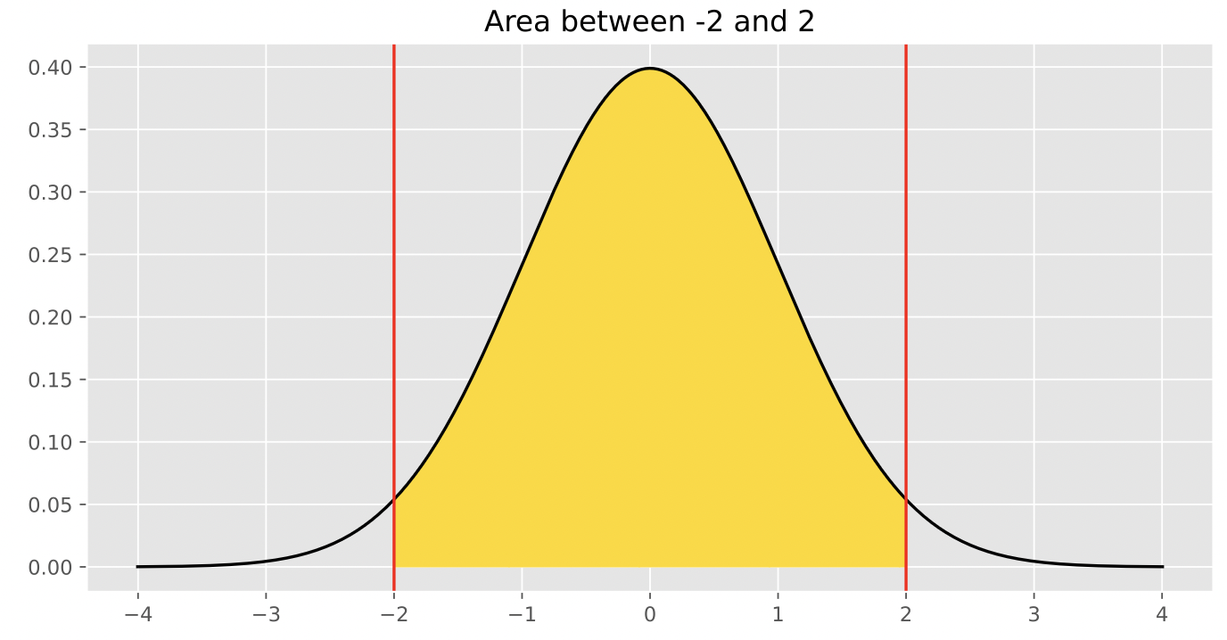
Given this information, it may be easier to express the problem as
“We draw a value from a normal distribution with mean 50 and SD 1.5.
What is the probability that the value is between 50 and 53?” Note that
this probability is equal to the proportion of values between 50
and 53 in a normal distribution whose mean is 50 and 1.5 (since
probabilities can be thought of as proportions).
In class, we typically worked with the standard normal
distribution, in which the mean was 0, the SD was 1, and the x-axis represented values in standard units.
Let’s convert the quantities of interest in this problem to standard
units, keeping in mind that the mean and SD we’re using now are the mean
and SD of the distribution of possible sample means, not of the
population.
50 converted to standard units is \frac{50
- \text{mean}}{\text{SD}} = \frac{50 - 50}{1.5} = 0 (no
calculation was necessary – 0 in standard units is equal to the mean in
original units).
53 converted to standard units is \frac{53
- \text{mean}}{\text{SD}} = \frac{53 - 50}{1.5} = 2.
Now, our problem boils down to finding the proportion of
values in a standard normal distribution that are between 0 and
2, or the proportion of values in a normal distribution
that are in the interval [\text{mean},
\text{mean} + 2 \text{ SDs}].
From class, we know that in a normal distribution, roughly 95% of
values are within 2 standard deviations of the mean, i.e. the proportion
of values in the interval [\text{mean} - 2
\text{ SDs}, \text{mean} + 2 \text{ SDs}] is 0.95.
Since the normal distribution is symmetric about the mean, half of
the values in this interval are to the right of the mean, and half are
to the left. This means that the proportion of values in the interval
[\text{mean}, \text{mean} + 2 \text{
SDs}] is \frac{0.95}{2} = 0.475,
which rounds to 0.48, and thus the desired result is 0.48.
Difficulty: ⭐️⭐️⭐️⭐️
The average score on this problem was 48%.
Problem 4
Lecture
17
The DataFrame apps contains application data for a
random sample of 1,000 applicants for a particular credit card from the
1990s. The "age" column contains the applicants’ ages, in
years, to the nearest twelfth of a year.
The credit card company that owns the data in apps,
BruinCard, has decided not to give us access to the entire
apps DataFrame, but instead just a random sample of 100
rows of apps called hundred_apps.
We are interested in estimating the mean age of all applicants in
apps given only the data in hundred_apps. The
ages in hundred_apps have a mean of 35 and a standard
deviation of 10.
Problem 4.1
Give the endpoints of the CLT-based 95% confidence interval for the
mean age of all applicants in apps, based on the data in
hundred_apps.
Answer: Left endpoint = 33, Right endpoint = 37
According to the Central Limit Theorem, the standard deviation of the
distribution of the sample mean is \frac{\text{sample SD}}{\sqrt{\text{sample size}}} =
\frac{10}{\sqrt{100}} = 1. Then using the fact that the
distribution of the sample mean is roughly normal, since 95% of the area
of a normal curve falls within two standard deviations of the mean, we
can find the endpoints of the 95% CLT-based confidence interval as 35 - 2 = 33 and 35
+ 2 = 37.
We can think of this as using the formula below:
\left[\text{sample mean} - 2\cdot \frac{\text{sample
SD}}{\sqrt{\text{sample size}}}, \: \text{sample mean} + 2\cdot
\frac{\text{sample SD}}{\sqrt{\text{sample size}}}
\right]. Plugging in the appropriate quantities yields [35 - 2\cdot\frac{10}{\sqrt{100}}, 35 -
2\cdot\frac{10}{\sqrt{100}}] = [33, 37].
Difficulty: ⭐️⭐️⭐️
The average score on this problem was 67%.
Problem 4.2
BruinCard reinstates our access to apps so that we can
now easily extract information about the ages of all applicants. We
determine that, just like in hundred_apps, the ages in
apps have a mean of 35 and a standard deviation of 10. This
raises the question of how other samples of 100 rows of
apps would have turned out, so we compute 10,000 sample means as follows.
sample_means = np.array([])for i in np.arange(10000): sample_mean = apps.sample(100, replace=True).get("age").mean() sample_means = np.append(sample_means, sample_mean)
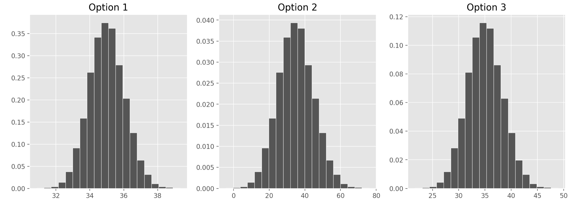
Which of the following three visualizations best depict the
distribution of sample_means?
Answer: Option 1
As we found in the previous part, the distribution of the sample mean
should have a standard deviation of 1. We also know it should be
centered at the mean of our sample, at 35, but since all the options are
centered here, that’s not too helpful. Only Option 1, however, has a
standard deviation of 1. Remember, we can approximate the standard
deviation of a normal curve as the distance between the mean and either
of the inflection points. Only Option 1 looks like it has inflection
points at 34 and 36, a distance of 1 from the mean of 35.
If you chose Option 2, you probably confused the standard deviation
of our original sample, 10, with the standard deviation of the
distribution of the sample mean, which comes from dividing that value by
the square root of the sample size.
Difficulty: ⭐️⭐️⭐️
The average score on this problem was 57%.
Problem 4.3
Which of the following statements are guaranteed to be true? Select
all that apply.
We used bootstrapping to compute sample_means.
The ages of credit card applicants are roughly normally
distributed.
A CLT-based 90% confidence interval for the mean age of credit card
applicants, based on the data in hundred apps, would be narrower than
the interval you gave in part (a).
The expression np.percentile(sample_means, 2.5)
evaluates to the left endpoint of the interval you gave in part (a).
If we used the data in hundred_apps to create 1,000
CLT-based 95% confidence intervals for the mean age of applicants in
apps, approximately 950 of them would contain the true mean
age of applicants in apps.
None of the above.
Answer: A CLT-based 90% confidence interval for the
mean age of credit card applicants, based on the data in
hundred_apps, would be narrower than the interval you gave
in part (a).
Let’s analyze each of the options:
Option 1: We are not using bootstrapping to compute sample means
since we are sampling from the apps DataFrame, which is our
population here. If we were bootstrapping, we’d need to sample from our
first sample, which is hundred_apps.
Option 2: We can’t be sure what the distribution of the ages of
credit card applicants are. The Central Limit Theorem says that the
distribution of sample_means is roughly normally
distributed, but we know nothing about the population
distribution.
Option 3: The CLT-based 95% confidence interval that we
calculated in part (a) was computed as follows: \left[\text{sample mean} - 2\cdot
\frac{\text{sample SD}}{\sqrt{\text{sample size}}},
\text{sample mean} + 2\cdot \frac{\text{sample SD}}{\sqrt{\text{sample
size}}}
\right] A CLT-based 90% confidence interval would be computed as
\left[\text{sample mean} - z\cdot
\frac{\text{sample SD}}{\sqrt{\text{sample size}}},
\text{sample mean} + z\cdot \frac{\text{sample SD}}{\sqrt{\text{sample
size}}}
\right] for some value of z less
than 2. We know that 95% of the area of a normal curve is within two
standard deviations of the mean, so to only pick up 90% of the area,
we’d have to go slightly less than 2 standard deviations away. This
means the 90% confidence interval will be narrower than the 95%
confidence interval.
Option 4: The left endpoint of the interval from part (a) was
calculated using the Central Limit Theorem, whereas using
np.percentile(sample_means, 2.5) is calculated empirically,
using the data in sample_means. Empirically calculating a
confidence interval doesn’t necessarily always give the exact same
endpoints as using the Central Limit Theorem, but it should give you
values close to those endpoints. These values are likely very similar
but they are not guaranteed to be the same. One way to see this is that
if we ran the code to generate sample_means again, we’d
probably get a different value for
np.percentile(sample_means, 2.5).
Option 5: The key observation is that if we used the data in
hundred_apps to create 1,000 CLT-based 95% confidence
intervals for the mean age of applicants in apps, all of
these intervals would be exactly the same. Given a sample, there is only
one CLT-based 95% confidence interval associated with it. In our case,
given the sample hundred_apps, the one and only CLT-based
95% confidence interval based on this sample is the one we found in part
(a). Therefore if we generated 1,000 of these intervals, either they
would all contain the parameter or none of them would. In order for a
statement like the one here to be true, we would need to collect 1,000
different samples, and calculate a confidence interval from each
one.
Difficulty: ⭐️⭐️⭐️⭐️
The average score on this problem was 49%.
Problem 5
Lecture
18
You need to estimate the proportion of American adults who want to be
vaccinated against Covid-19. You plan to survey a random sample of
American adults, and use the proportion of adults in your sample who
want to be vaccinated as your estimate for the true proportion in the
population. Your estimate must be within 0.04 of the true proportion,
95% of the time. Using the fact that the standard deviation of any
dataset of 0’s and 1’s is no more than 0.5, calculate the minimum number
of people you would need to survey. Input your answer below, as an
integer.
Answer: 625
Note: Before reviewing these solutions, it’s highly recommended
to revisit the lecture on “Choosing Sample Sizes,” since this problem
follows the main example from that lecture almost exactly.
While this solution is long, keep in mind from the start that our
goal is to solve for the smallest sample size necessary
to create a confidence interval that achieves certain criteria.
The Central Limit Theorem tells us that the distribution of the
sample mean is roughly normal, regardless of the distribution of the
population from which the samples are drawn. At first, it may not be
clear how the Central Limit Theorem is relevant, but remember that
proportions are means too – for instance, the proportion of adults who
want to be vaccinated is equal to the mean of a collection of 1s and 0s,
where we have a 1 for each adult that wants to be vaccinated and a 0 for
each adult who doesn’t want to be vaccinated. What this means (😉) is
that the Central Limit Theorem applies to the distribution of
the sample proportion, so we can use it here too.
Not only do we know that the distribution of sample proportions is
roughly normal, but we know its mean and standard deviation, too:
\begin{align*}
\text{Mean of Distribution of Possible Sample Means} &=
\text{Population Mean} = \text{Population Proportion} \\
\text{SD of Distribution of Possible Sample Means} &=
\frac{\text{Population SD}}{\sqrt{\text{Sample Size}}}
\end{align*}
Using this information, we can create a 95% confidence interval for
the population proportion, using the fact that in a normal distribution,
roughly 95% of values are within 2 standard deviations of the mean:
However, this interval depends on the population proportion (mean)
and SD, which we don’t know. (If we did know these parameters, there
would be no need to collect a sample!) Instead, we’ll use the sample
proportion and SD as rough estimates:
Note that the width of this interval – that is, its right endpoint
minus its left endpoint – is: \text{width} =
4 \cdot \frac{\text{Sample SD}}{\sqrt{\text{Sample Size}}}
In the problem, we’re told that we want our interval to be accurate
to within 0.04, which is equivalent to wanting the width of our interval
to be less than or equal to 0.08 (since the interval extends the same
amount above and below the sample proportion). As such, we need to pick
the smallest sample size necessary such that:
All we now need to do is pick the smallest sample size that satisfies
the above inequality. But there’s an issue – we don’t know what
our sample SD is, because we haven’t collected our sample!
Notice that in the inequality above, as the sample SD increases, so does
the minimum necessary sample size. In order to ensure we don’t collect
too small of a sample (which would result in the width of our confidence
interval being larger than desired), we can use an upper bound
for the SD of our sample. In the problem, we’re told that the largest
possible SD of a sample of 0s and 1s is 0.5 – this means that if we
replace our sample SD with 0.5, we will find a sample size such that the
width of our confidence interval is guaranteed to be less than or equal
to 0.08. This sample size may be larger than necessary, but that’s
better than it being smaller than necessary.
By substituting 0.5 for the sample SD in the last inequality above,
we get
We need to pick the smallest possible sample size that is greater
than or equal to 625; that’s just 625.
Difficulty: ⭐️⭐️⭐️⭐️
The average score on this problem was 40%.
Problem 6
Lecture
18
It’s your first time playing a new game called Brunch Menu.
The deck contains 96 cards, and each player will be dealt a hand of 9
cards. The goal of the game is to avoid having certain cards, called
Rotten Egg cards, which come with a penalty at the end of the
game. But you’re not sure how many of the 96 cards in the game are
Rotten Egg cards. So you decide to use the Central Limit
Theorem to estimate the proportion of Rotten Egg cards in the deck based
on the 9 random cards you are dealt in your hand.
Problem 6.1
You are dealt 3 Rotten Egg cards in your hand of 9 cards. You then
construct a CLT-based 95% confidence interval for the proportion of
Rotten Egg cards in the deck based on this sample. Approximately, how
wide is your confidence interval?
Choose the closest answer, and use the following facts:
The standard deviation of a collection of 0s and 1s is \sqrt{(\text{Prop. of 0s}) \cdot (\text{Prop of
1s})}.
\sqrt{18} is about \frac{17}{4}.
\frac{17}{9}
\frac{17}{27}
\frac{17}{81}
\frac{17}{96}
Answer:\frac{17}{27}
A Central Limit Theorem-based 95% confidence interval for a
population proportion is given by the following:
Note that this interval uses the fact that (about) 95% of values in a
normal distribution are within 2 standard deviations of the mean. It’s
key to divide by \sqrt{\text{Sample
Size}} when computing the standard deviation because the
distribution that is roughly normal is the distribution of the sample
mean (and hence, sample proportion), not the distribution of the sample
itself.
The width of the above interval – that is, the right endpoint minus
the left endpoint – is
Which of the following are limitations of trying to use the Central
Limit Theorem for this particular application? Select all that
apply.
The CLT is for large random samples, and our sample was not very
large.
The CLT is for random samples drawn with replacement, and our sample
was drawn without replacement.
The CLT is for normally distributed data, and our data may not have
been normally distributed.
The CLT is for sample means and sums, not sample proportions.
Answer: Options 1 and 2
Option 1: We use Central Limit Theorem (CLT) for
large random samples, and a sample of 9 is considered to be very small.
This makes it difficult to use CLT for this problem.
Option 2: Recall CLT happens when our sample is
drawn with replacement. When we are handed nine cards we are never
replacing cards back into our deck, which means that we are sampling
without replacement.
Option 3: This is wrong because CLT states that a
large sample is approximately a normal distribution even if the data
itself is not normally distributed. This means it doesn’t matter if our
data had not been normally distributed if we had a large enough sample
we could use CLT.
Option 4: This is wrong because CLT does apply to
the sample proportion distribution. Recall that proportions can be
treated like means.
Difficulty: ⭐️⭐️
The average score on this problem was 77%.
Problem 7
Lecture
18
You want to estimate the proportion of DSC majors who have a Netflix
subscription. To do so, you will survey a random sample of DSC majors
and ask them whether they have a Netflix subscription. You will then
create a 95% confidence interval for the proportion of “yes" answers in
the population, based on the responses in your sample. You decide that
your confidence interval should have a width of at most 0.10.
Problem 7.1
In order for your confidence interval to have a width of at most
0.10, the standard deviation of the distribution of the sample
proportion must be at most T. What is
T? Give your answer as an exact
decimal.
Answer: 0.025
Difficulty: ⭐️⭐️⭐️⭐️
The average score on this problem was 46%.
Problem 7.2
Using the fact that the standard deviation of any dataset of 0s and
1s is no more than 0.5, calculate the minimum number of people you would
need to survey so that the width of your confidence interval is at most
0.10. Give your answer as an integer.
Answer: 400
Difficulty: ⭐️⭐️
The average score on this problem was 81%.
Problem 8
Lecture
20
Arya was curious how many UCSD students used Hulu over Thanksgiving
break. He surveys 250 students and finds that 130 of them did use Hulu
over break and 120 did not.
Using this data, Arya decides to test following hypotheses:
Null Hypothesis: Over Thanksgiving break, an
equal number of UCSD students did use Hulu and did not use
Hulu.
Alternative Hypothesis: Over Thanksgiving break,
more UCSD students did use Hulu than did not use
Hulu.
Problem 8.1
Which of the following could be used as a test statistic for the
hypothesis test?
The proportion of students who did use Hulu minus the proportion of
students who did not use Hulu.
The absolute value of the proportion of students who did use Hulu
minus the proportion of students who did not use Hulu.
The proportion of students who did use Hulu plus the proportion of
students who did not use Hulu.
The absolute value of the proportion of students who did use Hulu
plus the proportion of students who did not use Hulu.
Answer: The proportion of students who did use Hulu
minus the proportion of students who did not use Hulu.
Difficulty: ⭐️⭐️
The average score on this problem was 81%.
Problem 8.2
For the test statistic that you chose in part (a), what is the
observed value of the statistic? Give your answer either as an exact
decimal or a simplified fraction.
Answer: 0.04
Difficulty: ⭐️
The average score on this problem was 90%.
Problem 8.3
If the p-value of the hypothesis test is 0.053, what can we conclude,
at the standard 0.05 significance level?
We reject the null hypothesis.
We fail to reject the null hypothesis.
We accept the null hypothesis.
Answer: We fail to reject the null hypothesis.
Difficulty: ⭐️⭐️
The average score on this problem was 87%.
Problem 9
Lecture
21
At the San Diego Model Railroad Museum, there are different admission
prices for children, adults, and seniors. Over a period of time, as
tickets are sold, employees keep track of how many of each type of
ticket are sold. These ticket counts (in the order child, adult, senior)
are stored as follows.
admissions_data = np.array([550, 1550, 400])
Problem 9.1
Complete the code below so that it creates an array
admissions_proportions with the proportions of tickets sold
to each group (in the order child, adult, senior).
To calculate proportion for each group, we divide each value in the
array (tickets sold to each group) by the sum of all values (total
tickets sold). Remember values in an array can be processed as a
whole.
Difficulty: ⭐️
The average score on this problem was 95%.
Problem 9.2
The museum employees have a model in mind for the proportions in
which they sell tickets to children, adults, and seniors. This model is
stored as follows.
model = np.array([0.25, 0.6, 0.15])
We want to conduct a hypothesis test to determine whether the
admissions data we have is consistent with this model. Which of the
following is the null hypothesis for this test?
Child, adult, and senior tickets might plausibly be purchased in
proportions 0.25, 0.6, and 0.15.
Child, adult, and senior tickets are purchased in proportions 0.25,
0.6, and 0.15.
Child, adult, and senior tickets might plausibly be purchased in
proportions other than 0.25, 0.6, and 0.15.
Child, adult, and senior tickets, are purchased in proportions other
than 0.25, 0.6, and 0.15.
Answer: Child, adult, and senior tickets are
purchased in proportions 0.25, 0.6, and 0.15. (Option 2)
Recall, null hypothesis is the hypothesis that there is no
significant difference between specified populations, any observed
difference being due to sampling or experimental error. So, we assume
the distribution is the same as the model.
Difficulty: ⭐️⭐️
The average score on this problem was 88%.
Problem 9.3
Which of the following test statistics could we use to test our
hypotheses? Select all that could work.
sum of differences in proportions
sum of squared differences in proportions
mean of differences in proportions
mean of squared differences in proportions
none of the above
Answer: sum of squared differences in proportions,
mean of squared differences in proportions (Option 2, 4)
We need to use squared difference to avoid the case that large
positive and negative difference cancel out in the process of
calculating sum or mean, resulting in small sum of difference or mean of
difference that does not reflect the actual deviation. So, we eliminate
Option 1 and 3.
Difficulty: ⭐️⭐️
The average score on this problem was 77%.
Problem 9.4
Below, we’ll perform the hypothesis test with a different test
statistic, the mean of the absolute differences in proportions.
Recall that the ticket counts we observed for children, adults, and
seniors are stored in the array
admissions_data = np.array([550, 1550, 400]), and that our
model is model = np.array([0.25, 0.6, 0.15]).
For our hypothesis test to determine whether the admissions data is
consistent with our model, what is the observed value of the test
statistic? Give your answer as a number between 0 and 1, rounded to
three decimal places. (Suppose that the value you calculated is assigned
to the variable observed_stat, which you will use in later
questions.)
Answer: 0.02
We first calculate the proportion for each value in
admissions_data\frac{550}{550+1550+400} = 0.22\frac{1550}{550+1550+400} = 0.62\frac{400}{550+1550+400} = 0.16 So, we have
the distribution of the admissions_data
Then, we calculate the observed value of the test statistic (the mean
of the absolute differences in proportions) \frac{|0.22-0.25|+|0.62-0.6|+|0.16-0.15|}{number\
of\ goups}=\frac{0.03+0.02+0.01}{3} =
0.02
Difficulty: ⭐️⭐️
The average score on this problem was 82%.
Problem 9.5
Now, we want to simulate the test statistic 10,000 times under the
assumptions of the null hypothesis. Fill in the blanks below to complete
this simulation and calculate the p-value for our hypothesis test.
Assume that the variables admissions_data,
admissions_proportions, model, and
observed_stat are already defined as specified earlier in
the question.
simulated_stats = np.array([]) for i in np.arange(10000): simulated_proportions = as_proportions(np.random.multinomial(__(a)__, __(b)__)) simulated_stat = __(c)__ simulated_stats = np.append(simulated_stats, simulated_stat)p_value = __(d)__
What goes in blank (a)? What goes in blank (b)? What goes in blank
(c)? What goes in blank (d)?
Recall, in np.random.multinomial(n, [p_1, ..., p_k]),
n is the number of experiments, and
[p_1, ..., p_k] is a sequence of probability. The method
returns an array of length k in which each element contains the number
of occurrences of an event, where the probability of the ith event is
p_i.
We want our simulated_proportion to have the same data
size as admissions_data, so we use
admissions_data.sum() in (a).
Since our null hypothesis is based on model, we simulate
based on distribution in model, so we have
model in (b).
In (c), we compute the mean of the absolute differences in
proportions. np.abs(simulated_proportions - model) gives us
a series of absolute differences, and .mean() computes the
mean of the absolute differences.
In (d), we calculate the p_value. Recall, the
p_value is the chance, under the null hypothesis, that the
test statistic is equal to the value that was observed in the data or is
even further in the direction of the alternative.
np.count_nonzero(simulated_stats >= observed_stat) gives
us the number of simulated_stats greater than or equal to
the observed_stat in the 10000 times simulations, so we
need to divide it by 10000 to compute the proportion of
simulated_stats greater than or equal to the
observed_stat, and this gives us the
p_value.
Difficulty: ⭐️⭐️
The average score on this problem was 79%.
Problem 9.6
True or False: the p-value represents the probability that the null
hypothesis is true.
True
False
Answer: False
Recall, the p-value is the chance, under the null hypothesis, that
the test statistic is equal to the value that was observed in the data
or is even further in the direction of the alternative. It only gives us
the strength of evidence in favor of the null hypothesis, which is
different from “the probability that the null hypothesis is true”.
Difficulty: ⭐️⭐️⭐️
The average score on this problem was 64%.
Problem 9.7
The new statistic that we used for this hypothesis test, the mean of
the absolute differences in proportions, is in fact closely related to
the total variation distance. Given two arrays of length three,
array_1 and array_2, suppose we compute the
mean of the absolute differences in proportions between
array_1 and array_2 and store the result as
madp. What value would we have to multiply
madp by to obtain the total variation distance
array_1 and array_2? Give your answer as a
number rounded to three decimal places.
Answer: 1.5
Recall, the total variation distance (TVD) is the sum of the absolute
differences in proportions, divided by 2. When we compute the mean of
the absolute differences in proportions, we are computing the sum of the
absolute differences in proportions, divided by the number of groups
(which is 3). Thus, to get TVD, we first multiply our current statistics
(the mean of the absolute differences in proportions) by 3, we get the
sum of the absolute differences in proportions. Then according to the
definition of TVD, we divide this value by 2. Thus, we have \text{current statistics}\cdot 3 / 2 = \text{current
statistics}\cdot 1.5.
Difficulty: ⭐️⭐️⭐️
The average score on this problem was 65%.
Problem 10
Lecture
20
For this question, let’s think of the data in app_data
as a random sample of all IKEA purchases and use it to test the
following hypotheses.
Null Hypothesis: IKEA sells an equal amount of beds
(category 'bed') and outdoor furniture (category
'outdoor').
Alternative Hypothesis: IKEA sells more beds than
outdoor furniture.
The DataFrame app_data contains 5000 rows, which form
our sample. Of these 5000 products,
1000 are beds,
1500 are outdoor furniture, and
2500 are in another category.
Problem 10.1
Which of the following could be used as the test
statistic for this hypothesis test? Select all that apply.
Among 2500 beds and outdoor furniture items, the absolute difference
between the proportion of beds and the proportion of outdoor
furniture.
Among 2500 beds and outdoor furniture items, the proportion of
beds.
Among 2500 beds and outdoor furniture items, the number of beds.
Among 2500 beds and outdoor furniture items, the number of beds plus
the number of outdoor furniture items.
Answer: Among 2500 beds and outdoor furniture
items, the proportion of beds. Among 2500 beds and outdoor
furniture items, the number of beds.
Our test statistic needs to be able to distinguish between the two
hypotheses. The first option does not do this, because it includes an
absolute value. If the absolute difference between the proportion of
beds and the proportion of outdoor furniture were large, it could be
because IKEA sells more beds than outdoor furniture, but it could also
be because IKEA sells more outdoor furniture than beds.
The second option is a valid test statistic, because if the
proportion of beds is large, that suggests that the alternative
hypothesis may be true.
Similarly, the third option works because if the number of beds (out
of 2500) is large, that suggests that the alternative hypothesis may be
true.
The fourth option is invalid because out of 2500 beds and outdoor
furniture items, the number of beds plus the number of outdoor furniture
items is always 2500. So the value of this statistic is constant
regardless of whether the alternative hypothesis is true, which means it
does not help you distinguish between the two hypotheses.
Difficulty: ⭐️⭐️
The average score on this problem was 78%.
Problem 10.2
Let’s do a hypothesis test with the following test statistic: among
2500 beds and outdoor furniture items, the proportion of outdoor
furniture minus the proportion of beds.
Complete the code below to calculate the observed value of the test
statistic and save the result as obs_diff.
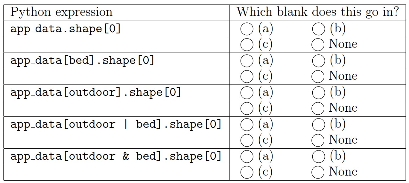
The table below contains several Python expressions. Choose the
correct expression to fill in each of the three blanks. Three
expressions will be used, and two will be unused.
Answer: Reading the table from top to bottom, the
five expressions should be used in the following blanks: None, (b), (a),
(c), None.
The first provided line of code defines a boolean Series called
outdoor with a value of True corresponding to
each outdoor furniture item in app_data. Using this as the
condition in a query results in a DataFrame of outdoor furniture items,
and using .shape[0] on this DataFrame gives the number of
outdoor furniture items. So app_data[outdoor].shape[0]
represents the number of outdoor furniture items in
app_data. Similarly, app_data[bed].shape[0]
represents the number of beds in app_data. Likewise,
app_data[outdoor | bed].shape[0] represents the total
number of outdoor furniture items and beds in app_data.
Notice that we need to use an or condition (|) to
get a DataFrame that contains both outdoor furniture and beds.
We are told that the test statistic should be the proportion of
outdoor furniture minus the proportion of beds. Translating this
directly into code, this means the test statistic should be calculated
as
Since this is a difference of two fractions with the same
denominator, we can equivalently subtract the numerators first, then
divide by the common denominator, using the mathematical fact \frac{a}{c} - \frac{b}{c} =
\frac{a-b}{c}.
Way 1 is a correct solution. This code begins by defining a variable
multi which will evaluate to an array with two elements
representing the number of items in each of the two categories, after
2500 items are drawn randomly from the two categories, with each
category being equally likely. In this case, our categories are beds and
outdoor furniture, and the null hypothesis says that each category is
equally likely, so this describes our scenario accurately. We can
interpret multi[0] as the number of outdoor furniture items
and multi[1] as the number of beds when we draw 2500 of
these items with equal probability. Using the same mathematical fact
from the solution to Problem 8.2, we can calculate the difference in
proportions as the difference in number divided by the total, so it is
correct to calculate the test statistic as
(multi[0] - multi[1])/2500.
Way 2 is an incorrect solution. Way 2 is based on a similar idea as
Way 1, except it calls np.random.multinomial twice, which
corresponds to two separate random processes of selecting 2500 items,
each of which is equally likely to be a bed or an outdoor furniture
item. However, is not guaranteed that the number of outdoor furniture
items in the first random selection plus the number of beds in the
second random selection totals 2500. Way 2 calculates the proportion of
outdoor furniture items in one random selection minus the proportion of
beds in another. What we want to do instead is calculate the difference
between the proportion of outdoor furniture and beds in a single random
draw.
Way 3 is a correct solution. Way 3 does the random selection of items
in a different way, using np.random.choice. Way 3 creates a
variable called choice which is an array of 2500 values.
Each value is chosen from the list [0,1] with each of the
two list elements being equally likely to be chosen. Of course, since we
are choosing 2500 items from a list of size 2, we must allow
replacements. We can interpret the elements of choice by
thinking of each 1 as an outdoor furniture item and each 0 as a bed. By
doing so, this random selection process matches up with the assumptions
of the null hypothesis. Then the sum of the elements of
choice represents the total number of outdoor furniture
items, which the code saves as the variable choice_sum.
Since there are 2500 beds and outdoor furniture items in total,
2500 - choice_sum represents the total number of beds.
Therefore, the test statistic here is correctly calculated as the number
of outdoor furniture items minus the number of beds, all divided by the
total number of items, which is 2500.
Way 4 is a correct solution. Way 4 is similar to Way 3, except
instead of using 0s and 1s, it uses the strings 'bed' and
'outdoor' in the choice array, so the
interpretation is even more direct. Another difference is the way the
number of beds and number of outdoor furniture items is calculated. It
uses np.count_nonzero instead of sum, which wouldn’t make
sense with strings. This solution calculates the proportion of outdoor
furniture minus the proportion of beds directly.
Way 5 is an incorrect solution. As described in the solution to
Problem 8.2, app_data[outdoor|bed] is a DataFrame
containing just the outdoor furniture items and the beds from
app_data. Based on the given information, we know
app_data[outdoor|bed] has 2500 rows, 1000 of which
correspond to beds and 1500 of which correspond to furniture items. This
code defines a variable samp that comes from sampling this
DataFrame 2500 times with replacement. This means that each row of
samp is equally likely to be any of the 2500 rows of
app_data[outdoor|bed]. The fraction of these rows that are
beds is 1000/2500 = 2/5 and the
fraction of these rows that are outdoor furniture items is 1500/2500 = 3/5. This means the random
process of selecting rows randomly such that each row is equally likely
does not make each item equally likely to be a bed or outdoor furniture
item. Therefore, this approach does not align with the assumptions of
the null hypothesis.
Way 6 is a correct solution. Way 6 essentially modifies Way 5 to make
beds and outdoor furniture items equally likely to be selected in the
random sample. As in Way 5, the code involves the DataFrame
app_data[outdoor|bed] which contains 1000 beds and 1500
outdoor furniture items. Then this DataFrame is grouped by
'category' which results in a DataFrame indexed by
'category', which will have only two rows, since there are
only two values of 'category', either
'outdoor' or 'bed'. The aggregation function
.count() is irrelevant here. When the index is reset,
'category' becomes a column. Now, randomly sampling from
this two-row grouped DataFrame such that each row is equally likely to
be selected does correspond to choosing items such that each
item is equally likely to be a bed or outdoor furniture item. The last
line simply calculates the proportion of outdoor furniture items minus
the proportion of beds in our random sample drawn according to the null
model.
Difficulty: ⭐️⭐️⭐️
The average score on this problem was 59%.
Problem 10.4
Suppose we generate 10,000 simulated values of the test statistic
according to the null model and store them in an array called
simulated_diffs. Complete the code below to calculate the
p-value for the hypothesis test.
To answer this question, we need to know whether small values or
large values of the test statistic indicate the alternative hypothesis.
The alternative hypothesis is that IKEA sells more beds than outdoor
furniture. Since we’re calculating the proportion of outdoor furniture
minus the proportion of beds, this difference will be small (negative)
if the alternative hypothesis is true. Larger (positive) values of the
test statistic mean that IKEA sells more outdoor furniture than beds. A
value near 0 means they sell beds and outdoor furniture equally.
The p-value is defined as the proportion of simulated test statistics
that are equal to the observed value or more extreme, where extreme
means in the direction of the alternative. In this case, since small
values of the test statistic indicate the alternative hypothesis, the
correct answer is <=.
Difficulty: ⭐️⭐️⭐️⭐️
The average score on this problem was 43%.
👋
Feedback: Find an error? Still confused? Have a suggestion?
Let us know
here.