← return to practice.dsc10.com
These problems are taken from past quizzes and exams. Work on them
on paper, since the quizzes and exams you take in this
course will also be on paper.
We encourage you to complete these
problems during discussion section. Solutions will be made available
after all discussion sections have concluded. You don’t need to submit
your answers anywhere.
Note: We do not plan to cover all of
these problems during the discussion section; the problems we don’t
cover can be used for extra practice.
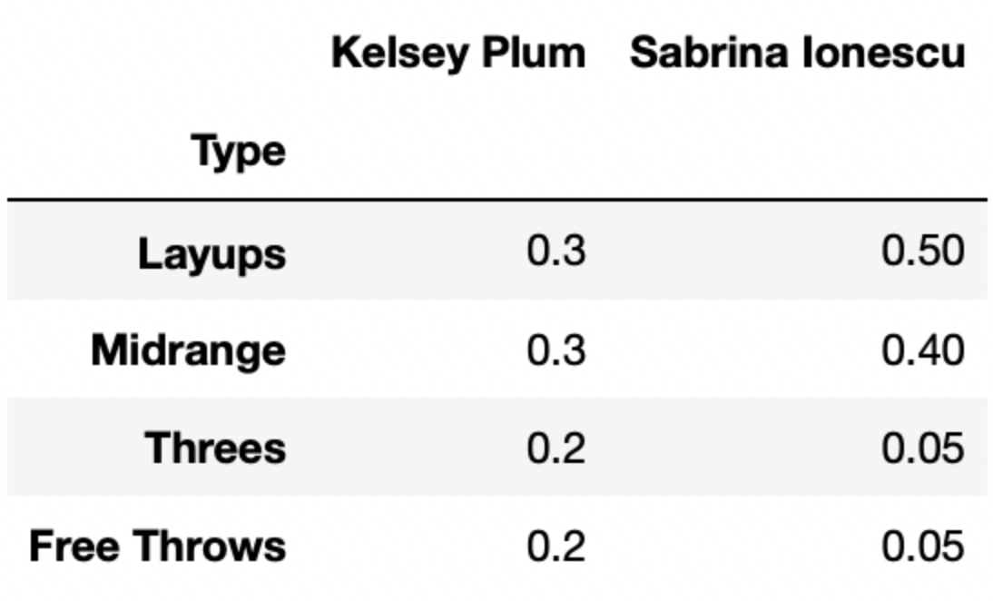
Let’s suppose there are 4 different types of shots a basketball player can take – layups, midrange shots, threes, and free throws.
The DataFrame breakdown has 4 rows and 50 columns – one
row for each of the 4 shot types mentioned above, and one column for
each of 50 different players. Each column of breakdown
describes the distribution of shot types for a single player.
The first few columns of breakdown are shown below.
For instance, 30% of Kelsey Plum’s shots are layups, 30% of her shots are midrange shots, 20% of her shots are threes, and 20% of her shots are free throws.
Below, we’ve drawn an overlaid bar chart showing the shot distributions of Kelsey Plum and Chiney Ogwumike, a player on the Los Angeles Sparks.
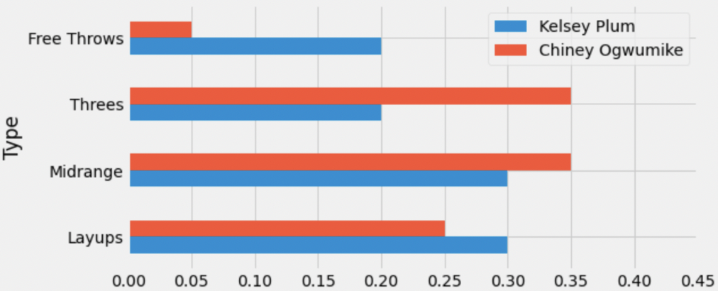
What is the total variation distance (TVD) between Kelsey Plum’s shot distribution and Chiney Ogwumike’s shot distribution? Give your answer as a proportion between 0 and 1 (not a percentage) rounded to three decimal places.
Answer: 0.2
Recall, the TVD is the sum of the absolute differences in proportions, divided by 2. The absolute differences in proportions for each category are as follows:
Then, we have
\text{TVD} = \frac{1}{2} (0.15 + 0.15 + 0.05 + 0.05) = 0.2
The average score on this problem was 84%.
Recall, breakdown has information for 50 different
players. We want to find the player whose shot distribution is the
most similar to Kelsey Plum, i.e. has the lowest TVD
with Kelsey Plum’s shot distribution.
Fill in the blanks below so that most_sim_player
evaluates to the name of the player with the most similar shot
distribution to Kelsey Plum. Assume that the column named
'Kelsey Plum' is the first column in breakdown
(and again that breakdown has 50 columns total).
most_sim_player = ''
lowest_tvd_so_far = __(a)__
other_players = np.array(breakdown.columns).take(__(b)__)
for player in other_players:
    player_tvd = tvd(breakdown.get('Kelsey Plum'),
                     breakdown.get(player))
    if player_tvd < lowest_tvd_so_far:
        lowest_tvd_so_far = player_tvd
__(c)__-1
-0.5
0
0.5
1
np.array([])
''
What goes in blank (b)?
What goes in blank (c)?
Answers: 1, np.arange(1, 50),
most_sim_player = player
Let’s try and understand the code provided to us. It appears that
we’re looping over the names of all other players, each time computing
the TVD between Kelsey Plum’s shot distribution and that player’s shot
distribution. If the TVD calculated in an iteration of the
for-loop (player_tvd) is less than the
previous lowest TVD (lowest_tvd_so_far), the current player
(player) is now the most “similar” to Kelsey Plum, and so
we store their TVD and name (in most_sim_player).
Before the for-loop, we haven’t looked at any other
players, so we don’t have values to store in
most_sim_player and lowest_tvd_so_far. On the
first iteration of the for-loop, both of these values need
to be updated to reflect Kelsey Plum’s similarity with the first player
in other_players. This is because, if we’ve only looked at
one player, that player is the most similar to Kelsey Plum.
most_sim_player is already initialized as an empty string,
and we will specify how to “update” most_sim_player in
blank (c). For blank (a), we need to pick a value of
lowest_tvd_so_far that we can guarantee
will be updated on the first iteration of the for-loop.
Recall, TVDs range from 0 to 1, with 0 meaning “most similar” and 1
meaning “most different”. This means that no matter what, the TVD
between Kelsey Plum’s distribution and the first player’s distribution
will be less than 1*, and so if we initialize
lowest_tvd_so_far to 1 before the for-loop, we
know it will be updated on the first iteration.
lowest_tvd_so_far and
most_sim_player wouldn’t be updated on the first iteration.
Rather, they’d be updated on the first iteration where
player_tvd is strictly less than 1. (We’d expect that the
TVDs between all pairs of players are neither exactly 0 nor exactly 1,
so this is not a practical issue.) To avoid this issue entirely, we
could change if player_tvd < lowest_tvd_so_far to
if player_tvd <= lowest_tvd_so_far, which would make
sure that even if the first TVD is 1, both
lowest_tvd_so_far and most_sim_player are
updated on the first iteration.lowest_tvd_so_far
to a value larger than 1 as well. Suppose we initialized it to 55 (an
arbitrary positive integer). On the first iteration of the
for-loop, player_tvd will be less than 55, and
so lowest_tvd_so_far will be updated.Then, we need other_players to be an array containing
the names of all players other than Kelsey Plum, whose name is stored at
position 0 in breakdown.columns. We are told that there are
50 players total, i.e. that there are 50 columns in
breakdown. We want to take the elements in
breakdown.columns at positions 1, 2, 3, …, 49 (the last
element), and the call to np.arange that generates this
sequence of positions is np.arange(1, 50). (Remember,
np.arange(a, b) does not include the second integer!)
In blank (c), as mentioned in the explanation for blank (a), we need
to update the value of most_sim_player. (Note that we only
arrive at this line if player_tvd is the lowest pairwise
TVD we’ve seen so far.) All this requires is
most_sim_player = player, since player
contains the name of the player who we are looking at in the current
iteration of the for-loop.
The average score on this problem was 70%.
You survey 100 DSC majors and 140 CSE majors to ask them which video streaming service they use most. The resulting distributions are given in the table below. Note that each column sums to 1.
| Service | DSC Majors | CSE Majors |
|---|---|---|
| Netflix | 0.4 | 0.35 |
| Hulu | 0.25 | 0.2 |
| Disney+ | 0.1 | 0.1 |
| Amazon Prime Video | 0.15 | 0.3 |
| Other | 0.1 | 0.05 |
For example, 20% of CSE Majors said that Hulu is their most used video streaming service. Note that if a student doesn’t use video streaming services, their response is counted as Other.
What is the total variation distance (TVD) between the distribution for DSC majors and the distribution for CSE majors? Give your answer as an exact decimal.
Answer: 0.15
The average score on this problem was 89%.
Suppose we only break down video streaming services into four categories: Netflix, Hulu, Disney+, and Other (which now includes Amazon Prime Video). Now we recalculate the TVD between the two distributions. How does the TVD now compare to your answer to part (a)?
less than (a)
equal to (a)
greater than (a)
Answer: less than (a)
The average score on this problem was 93%.
In some cities, the number of sunshine hours per month is relatively consistent throughout the year. São Paulo, Brazil is one such city; in all months of the year, the number of sunshine hours per month is somewhere between 139 and 173. New York City’s, on the other hand, ranges from 139 to 268.
Gina and Abel, both San Diego natives, are interested in assessing how “consistent" the number of sunshine hours per month in San Diego appear to be. Specifically, they’d like to test the following hypotheses:
Null Hypothesis: The number of sunshine hours per month in San Diego is drawn from the uniform distribution, \left[\frac{1}{12}, \frac{1}{12}, ..., \frac{1}{12}\right]. (In other words, the number of sunshine hours per month in San Diego is equal in all 12 months of the year.)
Alternative Hypothesis: The number of sunshine hours per month in San Diego is not drawn from the uniform distribution.
As their test statistic, Gina and Abel choose the total variation distance. To simulate samples under the null, they will sample from a categorical distribution with 12 categories — January, February, and so on, through December — each of which have an equal probability of being chosen.
In order to run their hypothesis test, Gina and Abel need a way to calculate their test statistic. Below is an incomplete implementation of a function that computes the TVD between two arrays of length 12, each of which represent a categorical distribution.
    def calculate_tvd(dist1, dist2):
        return np.mean(np.abs(dist1 - dist2)) * ____
Fill in the blank so that calculate_tvd works as
intended.
1 / 6
1 / 3
1 / 2
2
3
6
Answer: 6
The TVD is the sum of the absolute differences in proportions,
divided by 2. In the code to the left of the blank, we’ve computed the
mean of the absolute differences in proportions, which is the same as
the sum of the absolute differences in proportions, divided by 12 (since
len(dist1) is 12). To correct the fact that we
divided by 12, we multiply by 6, so that we’re only dividing by 2.
The average score on this problem was 17%.
Moving forward, assume that calculate_tvd works
correctly.
Now, complete the implementation of the function
uniform_test, which takes in an array
observed_counts of length 12 containing the number of
sunshine hours each month in a city and returns the p-value for the
hypothesis test stated at the start of the question.
    def uniform_test(observed_counts):
        # The values in observed_counts are counts, not proportions!
        total_count = observed_counts.sum()
        uniform_dist = __(b)__
        tvds = np.array([])
        for i in np.arange(10000):
            simulated = __(c)__
            tvd = calculate_tvd(simulated, __(d)__)
            tvds = np.append(tvds, tvd)
return np.mean(tvds __(e)__ calculate_tvd(uniform_dist, __(f)__))What goes in blank (b)? (Hint: The function
np.ones(k) returns an array of length k in
which all elements are 1.)
Answer: np.ones(12) / 12
uniform_dist needs to be the same as the uniform
distribution provided in the null hypothesis, \left[\frac{1}{12}, \frac{1}{12}, ...,
\frac{1}{12}\right].
In code, this is an array of length 12 in which each element is equal
to 1 / 12. np.ones(12)
creates an array of length 12 in which each value is 1; for
each value to be 1 / 12, we divide np.ones(12)
by 12.
The average score on this problem was 66%.
What goes in blank (c)?
np.random.multinomial(12, uniform_dist)
np.random.multinomial(12, uniform_dist) / 12
np.random.multinomial(12, uniform_dist) / total_count
np.random.multinomial(total_count, uniform_dist)
np.random.multinomial(total_count, uniform_dist) / 12
np.random.multinomial(total_count, uniform_dist) / total_count
Answer:
np.random.multinomial(total_count, uniform_dist) / total_count
The idea here is to repeatedly generate an array of proportions that
results from distributing total_count hours across the 12
months in a way that each month is equally likely to be chosen. Each
time we generate such an array, we’ll determine its TVD from the uniform
distribution; doing this repeatedly gives us an empirical distribution
of the TVD under the assumption the null hypothesis is true.
The average score on this problem was 21%.
What goes in blank (d)?
Answer: uniform_dist
As mentioned above:
Each time we generate such an array, we’ll determine its TVD from the uniform distribution; doing this repeatedly gives us an empirical distribution of the TVD under the assumption the null hypothesis is true.
The average score on this problem was 54%.
What goes in blank (e)?
>
>=
<
<=
==
!=
Answer: >=
The purpose of the last line of code is to compute the p-value for the hypothesis test. Recall, the p-value of a hypothesis test is the proportion of simulated test statistics that are as or more extreme than the observed test statistic, under the assumption the null hypothesis is true. In this context, “as extreme or more extreme” means the simulated TVD is greater than or equal to the observed TVD (since larger TVDs mean “more different”).
The average score on this problem was 77%.
What goes in blank (f)?
Answer: observed_counts / total_count
or observed_counts / observed_counts.sum()
Blank (f) needs to contain the observed distribution of sunshine hours (as an array of proportions) that we compare against the uniform distribution to calculate the observed TVD. This observed TVD is then compared with the distribution of simulated TVDs to calculate the p-value. The observed counts are converted to proportions by dividing by the total count so that the observed distribution is on the same scale as the simulated and expected uniform distributions, which are also in proportions.
The average score on this problem was 27%.
Kelsey Plum, a WNBA player, attended La Jolla Country Day School,
which is adjacent to UCSD’s campus. Her current team is the Las Vegas
Aces (three-letter code 'LVA'). In 2021, the Las
Vegas Aces played 31 games, and Kelsey Plum played in all
31.
The DataFrame plum contains her stats for all games the
Las Vegas Aces played in 2021. The first few rows of plum
are shown below (though the full DataFrame has 31 rows, not 5):

Each row in plum corresponds to a single game. For each
game, we have:
'Date' (str), the date on which the game
was played'Opp' (str), the three-letter code of the
opponent team'Home' (bool), True if the
game was played in Las Vegas (“home”) and False if it was
played at the opponent’s arena (“away”)'Won' (bool), True if the Las
Vegas Aces won the game and False if they lost'PTS' (int), the number of points Kelsey
Plum scored in the game'AST' (int), the number of assists
(passes) Kelsey Plum made in the game'TOV' (int), the number of turnovers
Kelsey Plum made in the game (a turnover is when you lose the ball –
turnovers are bad!) Consider the definition of the function
diff_in_group_means:
def diff_in_group_means(df, group_col, num_col):
    s = df.groupby(group_col).mean().get(num_col)
return s.loc[False] - s.loc[True]It turns out that Kelsey Plum averages 0.61 more assists in games
that she wins (“winning games”) than in games that she loses (“losing
games”). Fill in the blanks below so that observed_diff
evaluates to -0.61.
observed_diff = diff_in_group_means(plum, __(a)__, __(b)__)What goes in blank (a)?
What goes in blank (b)?
Answers: 'Won', 'AST'
To compute the number of assists Kelsey Plum averages in winning and
losing games, we need to group by 'Won'. Once doing so, and
using the .mean() aggregation method, we need to access
elements in the 'AST' column.
The second argument to diff_in_group_means,
group_col, is the column we’re grouping by, and so blank
(a) must be filled by 'Won'. Then, the second argument,
num_col, must be 'AST'.
Note that after extracting the Series containing the average number
of assists in wins and losses, we are returning the value with the index
False (“loss”) minus the value with the index
True (“win”). So, throughout this problem, keep in mind
that we are computing “losses minus wins”. Since our observation was
that she averaged 0.61 more assists in wins than in losses, it makes
sense that diff_in_group_means(plum, 'Won', 'AST') is -0.61
(rather than +0.61).
The average score on this problem was 94%.
After observing that Kelsey Plum averages more assists in winning games than in losing games, we become interested in conducting a permutation test for the following hypotheses:
To conduct our permutation test, we place the following code in a
for-loop.
won = plum.get('Won')
ast = plum.get('AST')
shuffled = plum.assign(Won_shuffled=np.random.permutation(won)) \
               .assign(AST_shuffled=np.random.permutation(ast))
Which of the following options does not compute a valid simulated test statistic for this permutation test?
diff_in_group_means(shuffled, 'Won', 'AST')
diff_in_group_means(shuffled, 'Won', 'AST_shuffled')
diff_in_group_means(shuffled, 'Won_shuffled, 'AST')
diff_in_group_means(shuffled, 'Won_shuffled, 'AST_shuffled')
More than one of these options do not compute a valid simulated test statistic for this permutation test
Answer:
diff_in_group_means(shuffled, 'Won', 'AST')
As we saw in the previous subpart,
diff_in_group_means(shuffled, 'Won', 'AST') computes the
observed test statistic, which is -0.61. There is no randomness involved
in the observed test statistic; each time we run the line
diff_in_group_means(shuffled, 'Won', 'AST') we will see the
same result, so this cannot be used for simulation.
To perform a permutation test here, we need to simulate under the null by randomly assigning assist counts to groups; here, the groups are “win” and “loss”.
As such, Options 2 through 4 are all valid, and Option 1 is the only invalid one.
The average score on this problem was 68%.
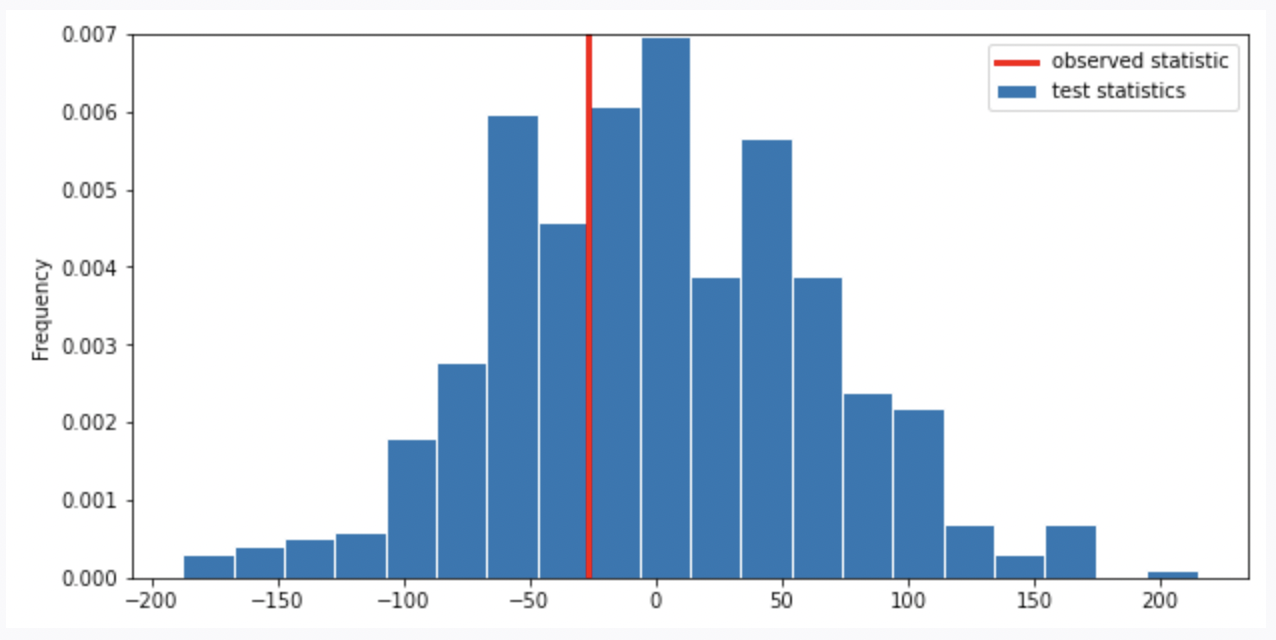
Suppose we generate 10,000 simulated test statistics, using one of
the valid options from part 1. The empirical distribution of test
statistics, with a red line at observed_diff, is shown
below.
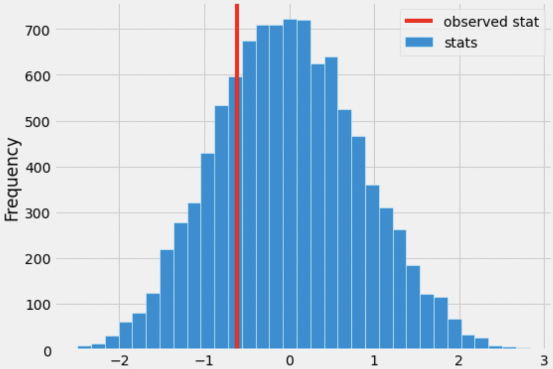
Roughly one-quarter of the area of the histogram above is to the left of the red line. What is the correct interpretation of this result?
There is roughly a one quarter probability that Kelsey Plum’s number of assists in winning games and in losing games come from the same distribution.
The significance level of this hypothesis test is roughly a quarter.
Under the assumption that Kelsey Plum’s number of assists in winning games and in losing games come from the same distribution, and that she wins 22 of the 31 games she plays, the chance of her averaging at least 0.61 more assists in wins than losses is roughly a quarter.
Under the assumption that Kelsey Plum’s number of assists in winning games and in losing games come from the same distribution, and that she wins 22 of the 31 games she plays, the chance of her averaging 0.61 more assists in wins than losses is roughly a quarter.
Answer: Under the assumption that Kelsey Plum’s number of assists in winning games and in losing games come from the same distribution, and that she wins 22 of the 31 games she plays, the chance of her averaging at least 0.61 more assists in wins than losses is roughly a quarter. (Option 3)
First, we should note that the area to the left of the red line (a quarter) is the p-value of our hypothesis test. Generally, the p-value is the probability of observing an outcome as or more extreme than the observed, under the assumption that the null hypothesis is true. The direction to look in depends on the alternate hypothesis; here, since our alternative hypothesis is that the number of assists Kelsey Plum makes in winning games is higher on average than in losing games, a “more extreme” outcome is where the assists in winning games are higher than in losing games, i.e. where \text{(assists in wins)} - \text{(assists in losses)} is positive or where \text{(assists in losses)} - \text{(assists in wins)} is negative. As mentioned in the solution to the first subpart, our test statistic is \text{(assists in losses)} - \text{(assists in wins)}, so a more extreme outcome is one where this is negative, i.e. to the left of the observed statistic.
Let’s first rule out the first two options.
Now, the only difference between Options 3 and 4 is the inclusion of “at least” in Option 3. Remember, to compute a p-value we must compute the probability of observing something as or more extreme than the observed, under the null. The “or more” corresponds to “at least” in Option 3. As such, Option 3 is the correct choice.
The average score on this problem was 70%.
app_data has a row for each product build that
was logged on the app. The column 'product' contains the
name of the product, and the column 'minutes' contains
integer values representing the number of minutes it took to assemble
each product. You are browsing the IKEA showroom, deciding whether to purchase the
BILLY bookcase or the LOMMARP bookcase. You are concerned about the
amount of time it will take to assemble your new bookcase, so you look
up the assembly times reported in app_data. Thinking of the
data in app_data as a random sample of all IKEA purchases,
you want to perform a permutation test to test the following
hypotheses.
Null Hypothesis: The assembly time for the BILLY bookcase and the assembly time for the LOMMARP bookcase come from the same distribution.
Alternative Hypothesis: The assembly time for the BILLY bookcase and the assembly time for the LOMMARP bookcase come from different distributions.
Suppose we query app_data to keep only the BILLY
bookcases, then average the 'minutes' column. In addition,
we separately query app_data to keep only the LOMMARP
bookcases, then average the 'minutes' column. If the null
hypothesis is true, which of the following statements about these two
averages is correct?
These two averages are the same.
Any difference between these two averages is due to random chance.
Any difference between these two averages cannot be ascribed to random chance alone.
The difference between these averages is statistically significant.
Answer: Any difference between these two averages is due to random chance.
If the null hypothesis is true, this means that the time recorded in
app_data for each BILLY bookcase is a random number that
comes from some distribution, and the time recorded in
app_data for each LOMMARP bookcase is a random number that
comes from the same distribution. Each assembly time is a
random number, so even if the null hypothesis is true, if we take one
person who assembles a BILLY bookcase and one person who assembles a
LOMMARP bookcase, there is no guarantee that their assembly times will
match. Their assembly times might match, or they might be different,
because assembly time is random. Randomness is the only reason that
their assembly times might be different, as the null hypothesis says
there is no systematic difference in assembly times between the two
bookcases. Specifically, it’s not the case that one typically takes
longer to assemble than the other.
With those points in mind, let’s go through the answer choices.
The first answer choice is incorrect. Just because two sets of
numbers are drawn from the same distribution, the numbers themselves
might be different due to randomness, and the averages might also be
different. Maybe just by chance, the people who assembled the BILLY
bookcases and recorded their times in app_data were slower
on average than the people who assembled LOMMARP bookcases. If the null
hypothesis is true, this difference in average assembly time should be
small, but it very likely exists to some degree.
The second answer choice is correct. If the null hypothesis is true, the only reason for the difference is random chance alone.
The third answer choice is incorrect for the same reason that the second answer choice is correct. If the null hypothesis is true, any difference must be explained by random chance.
The fourth answer choice is incorrect. If there is a difference between the averages, it should be very small and not statistically significant. In other words, if we did a hypothesis test and the null hypothesis was true, we should fail to reject the null.
The average score on this problem was 77%.
For the permutation test, we’ll use as our test statistic the average assembly time for BILLY bookcases minus the average assembly time for LOMMARP bookcases, in minutes.
Complete the code below to generate one simulated value of the test
statistic in a new way, without using
np.random.permutation.
billy = (app_data.get('product') ==
        'BILLY Bookcase, white, 31 1/2x11x79 1/2')
lommarp = (app_data.get('product') ==
          'LOMMARP Bookcase, dark blue-green, 25 5/8x78 3/8')
billy_lommarp = app_data[billy|lommarp]
billy_mean = np.random.choice(billy_lommarp.get('minutes'), billy.sum(), replace=False).mean()
lommarp_mean = _________
billy_mean - lommarp_mean
What goes in the blank?
billy_lommarp[lommarp].get('minutes').mean()
np.random.choice(billy_lommarp.get('minutes'), lommarp.sum(), replace=False).mean()
billy_lommarp.get('minutes').mean() - billy_mean
(billy_lommarp.get('minutes').sum() - billy_mean * billy.sum())/lommarp.sum()
Answer:
(billy_lommarp.get('minutes').sum() - billy_mean * billy.sum())/lommarp.sum()
The first line of code creates a boolean Series with a True value for
every BILLY bookcase, and the second line of code creates the analogous
Series for the LOMMARP bookcase. The third line queries to define a
DataFrame called billy_lommarp containing all products that
are BILLY or LOMMARP bookcases. In other words, this DataFrame contains
a mix of BILLY and LOMMARP bookcases.
From this point, the way we would normally proceed in a permutation
test would be to use np.random.permutation to shuffle one
of the two relevant columns (either 'product' or
'minutes') to create a random pairing of assembly times
with products. Then we would calculate the average of all assembly times
that were randomly assigned to the label BILLY. Similarly, we’d
calculate the average of all assembly times that were randomly assigned
to the label LOMMARP. Then we’d subtract these averages to get one
simulated value of the test statistic. To run the permutation test, we’d
have to repeat this process many times.
In this problem, we need to generate a simulated value of the test
statistic, without randomly shuffling one of the columns. The code
starts us off by defining a variable called billy_mean that
comes from using np.random.choice. There’s a lot going on
here, so let’s break it down. Remember that the first argument to
np.random.choice is a sequence of values to choose from,
and the second is the number of random choices to make. And we set
replace=False, so that no element that has already been
chosen can be chosen again. Here, we’re making our random choices from
the 'minutes' column of billy_lommarp. The
number of choices to make from this collection of values is
billy.sum(), which is the sum of all values in the
billy Series defined in the first line of code. The
billy Series contains True/False values, but in Python,
True counts as 1 and False counts as 0, so billy.sum()
evaluates to the number of True entries in billy, which is
the number of BILLY bookcases recorded in app_data. It
helps to think of the random process like this:
If we think of the random times we draw as being labeled BILLY, then the remaining assembly times still leftover in the bag represent the assembly times randomly labeled LOMMARP. In other words, this is a random association of assembly times to labels (BILLY or LOMMARP), which is the same thing we usually accomplish by shuffling in a permutation test.
From here, we can proceed the same way as usual. First, we need to
calculate the average of all assembly times that were randomly assigned
to the label BILLY. This is done for us and stored in
billy_mean. We also need to calculate the average of all
assembly times that were randomly assigned the label LOMMARP. We’ll call
that lommarp_mean. Thinking of picking times out of a large
bag, this is the average of all the assembly times left in the bag. The
problem is there is no easy way to access the assembly times that were
not picked. We can take advantage of the fact that we can easily
calculate the total assembly time of all BILLY and LOMMARP bookcases
together with billy_lommarp.get('minutes').sum(). Then if
we subtract the total assembly time of all bookcases randomly labeled
BILLY, we’ll be left with the total assembly time of all bookcases
randomly labeled LOMMARP. That is,
billy_lommarp.get('minutes').sum() - billy_mean * billy.sum()
represents the total assembly time of all bookcases randomly labeled
LOMMARP. The count of the number of LOMMARP bookcases is given by
lommarp.sum() so the average is
(billy_lommarp.get('minutes').sum() - billy_mean * billy.sum())/lommarp.sum().
A common wrong answer for this question was the second answer choice,
np.random.choice(billy_lommarp.get('minutes'), lommarp.sum(), replace=False).mean().
This mimics the structure of how billy_mean was defined so
it’s a natural guess. However, this corresponds to the following random
process, which doesn’t associate each assembly with a unique label
(BILLY or LOMMARP):
We could easily get the same assembly time once for BILLY and once for LOMMARP, while other assembly times could get picked for neither. This process doesn’t split the data into two random groups as desired.
The average score on this problem was 12%.
apps contains application
data for a random sample of 1,000 applicants for a particular credit
card from the 1990s. The columns are:
"status" (str): Whether the credit card application
was approved: "approved" or "denied" values
only.
"age" (float): The applicant’s age, in years, to the
nearest twelfth of a year.
"income" (float): The applicant’s annual income, in
tens of thousands of dollars.
"homeowner" (str): Whether the credit card applicant
owns their own home: "yes" or "no" values
only.
"dependents" (int): The number of dependents, or
individuals that rely on the applicant as a primary source of income,
such as children.
The first few rows of apps are shown below, though
remember that apps has 1,000 rows.
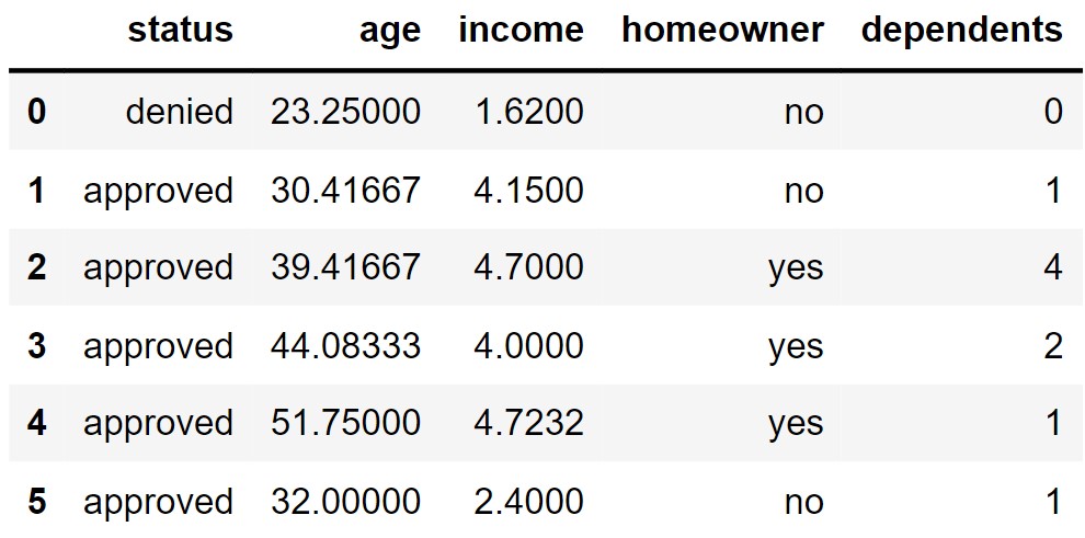
In apps, our sample of 1,000 credit card applications,
applicants who were approved for the credit card have fewer dependents,
on average, than applicants who were denied. The mean number of
dependents for approved applicants is 0.98, versus 1.07 for denied
applicants.
To test whether this difference is purely due to random chance, or whether the distributions of the number of dependents for approved and denied applicants are truly different in the population of all credit card applications, we decide to perform a permutation test.
Consider the incomplete code block below.
def shuffle_status(df):
    shuffled_status = np.random.permutation(df.get("status"))
    return df.assign(status=shuffled_status).get(["status", "dependents"])

def test_stat(df):
    grouped = df.groupby("status").mean().get("dependents")
    approved = grouped.loc["approved"]
    denied = grouped.loc["denied"]
    return __(a)__

stats = np.array([])
for i in np.arange(10000):
    shuffled_apps = shuffle_status(apps)
    stat = test_stat(shuffled_apps)
    stats = np.append(stats, stat)

p_value = np.count_nonzero(__(b)__) / 10000
Below are six options for filling in blanks (a) and (b) in the code above.
| Blank (a) | Blank (b) | |
|---|---|---|
| Option 1 | denied - approved |
stats >= test_stat(apps) |
| Option 2 | denied - approved |
stats <= test_stat(apps) |
| Option 3 | approved - denied |
stats >= test_stat(apps) |
| Option 4 | np.abs(denied - approved) |
stats >= test_stat(apps) |
| Option 5 | np.abs(denied - approved) |
stats <= test_stat(apps) |
| Option 6 | np.abs(approved - denied) |
stats >= test_stat(apps) |
The correct way to fill in the blanks depends on how we choose our null and alternative hypotheses.
Suppose we choose the following pair of hypotheses.
Null Hypothesis: In the population, the number of dependents of approved and denied applicants come from the same distribution.
Alternative Hypothesis: In the population, the number of dependents of approved applicants and denied applicants do not come from the same distribution.
Which of the six presented options could correctly fill in blanks (a) and (b) for this pair of hypotheses? Select all that apply.
Option 1
Option 2
Option 3
Option 4
Option 5
Option 6
None of the above.
Answer: Option 4, Option 6
For blank (a), we want to choose a test statistic that helps us
distinguish between the null and alternative hypotheses. The alternative
hypothesis says that denied and approved
should be different, but it doesn’t say which should be larger. Options
1 through 3 therefore won’t work, because high values and low values of
these statistics both point to the alternative hypothesis, and moderate
values point to the null hypothesis. Options 4 through 6 all work
because large values point to the alternative hypothesis, and small
values close to 0 suggest that the null hypothesis should be true.
For blank (b), we want to calculate the p-value in such a way that it
represents the proportion of trials for which the simulated test
statistic was equal to the observed statistic or further in the
direction of the alternative. For all of Options 4 through 6, large
values of the test statistic indicate the alternative, so we need to
calculate the p-value with a >= sign, as in Options 4
and 6.
While Option 3 filled in blank (a) correctly, it did not fill in blank (b) correctly. Options 4 and 6 fill in both blanks correctly.
The average score on this problem was 78%.
Now, suppose we choose the following pair of hypotheses.
Null Hypothesis: In the population, the number of dependents of approved and denied applicants come from the same distribution.
Alternative Hypothesis: In the population, the number of dependents of approved applicants is smaller on average than the number of dependents of denied applicants.
Which of the six presented options could correctly fill in blanks (a) and (b) for this pair of hypotheses? Select all that apply.
Answer: Option 1
As in the previous part, we need to fill blank (a) with a test
statistic such that large values point towards one of the hypotheses and
small values point towards the other. Here, the alterntive hypothesis
suggests that approved should be less than
denied, so we can’t use Options 4 through 6 because these
can only detect whether approved and denied
are not different, not which is larger. Any of Options 1 through 3
should work, however. For Options 1 and 2, large values point towards
the alternative, and for Option 3, small values point towards the
alternative. This means we need to calculate the p-value in blank (b)
with a >= symbol for the test statistic from Options 1
and 2, and a <= symbol for the test statistic from
Option 3. Only Options 1 fills in blank (b) correctly based on the test
statistic used in blank (a).
The average score on this problem was 83%.
Option 6 from the start of this question is repeated below.
| Blank (a) | Blank (b) | |
|---|---|---|
| Option 6 | np.abs(approved - denied) |
stats >= test_stat(apps) |
We want to create a new option, Option 7, that replicates the behavior of Option 6, but with blank (a) filled in as shown:
| Blank (a) | Blank (b) | |
|---|---|---|
| Option 7 | approved - denied |
Which expression below could go in blank (b) so that Option 7 is equivalent to Option 6?
np.abs(stats) >= test_stat(apps)
stats >= np.abs(test_stat(apps))
np.abs(stats) >= np.abs(test_stat(apps))
np.abs(stats >= test_stat(apps))
Answer:
np.abs(stats) >= np.abs(test_stat(apps))
First, we need to understand how Option 6 works. Option 6 produces
large values of the test statistic when approved is very
different from denied, then calculates the p-value as the
proportion of trials for which the simulated test statistic was larger
than the observed statistic. In other words, Option 6 calculates the
proportion of trials in which approved and
denied are more different in a pair of random samples than
they are in the original samples.
For Option 7, the test statistic for a pair of random samples may
come out very large or very small when approved is very
different from denied. Similarly, the observed statistic
may come out very large or very small when approved and
denied are very different in the original samples. We want
to find the proportion of trials in which approved and
denied are more different in a pair of random samples than
they are in the original samples, which means we want the proportion of
trials in which the absolute value of approved - denied in
a pair of random samples is larger than the absolute value of
approved - denied in the original samples.
The average score on this problem was 56%.
In our implementation of this permutation test, we followed the
procedure outlined in lecture to draw new pairs of samples under the
null hypothesis and compute test statistics — that is, we randomly
assigned each row to a group (approved or denied) by shuffling one of
the columns in apps, then computed the test statistic on
this random pair of samples.
Let’s now explore an alternative solution to drawing pairs of samples under the null hypothesis and computing test statistics. Here’s the approach:
"dependents"
column as the new “denied” sample, and the values at the at the bottom
of the resulting "dependents" column as the new “approved”
sample. Note that we don’t necessarily split the DataFrame exactly in
half — the sizes of these new samples depend on the number of “denied”
and “approved” values in the original DataFrame!Once we generate our pair of random samples in this way, we’ll compute the test statistic on the random pair, as usual. Here, we’ll use as our test statistic the difference between the mean number of dependents for denied and approved applicants, in the order denied minus approved.
Fill in the blanks to complete the simulation below.
Hint: np.random.permutation shouldn’t appear
anywhere in your code.
    def shuffle_all(df):
        '''Returns a DataFrame with the same rows as df, but reordered.'''
        return __(a)__

    def fast_stat(df):
        # This function does not and should not contain any randomness.
        denied = np.count_nonzero(df.get("status") == "denied")
        mean_denied = __(b)__.get("dependents").mean()
        mean_approved = __(c)__.get("dependents").mean()
        return mean_denied - mean_approved

    stats = np.array([])
    for i in np.arange(10000):
        stat = fast_stat(shuffle_all(apps))
stats = np.append(stats, stat)Answer: The blanks should be filled in as follows:
df.sample(df.shape[0])df.take(np.arange(denied))df.take(np.arange(denied, df.shape[0]))For blank (a), we are told to return a DataFrame with the same rows
but in a different order. We can use the .sample method for
this question. We want each row of the input DataFrame df
to appear once, so we should sample without replacement, and we should
have has many rows in the output as in df, so our sample
should be of size df.shape[0]. Since sampling without
replacement is the default behavior of .sample, it is
optional to specify replace=False.
The average score on this problem was 59%.
For blank (b), we need to implement the strategy outlined, where
after we shuffle the DataFrame, we use the values at the top of the
DataFrame as our new “denied sample. In a permutation test, the two
random groups we create should have the same sizes as the two original
groups we are given. In this case, the size of the”denied” group in our
original data is stored in the variable denied. So we need
the rows in positions 0, 1, 2, …, denied - 1, which we can
get using df.take(np.arange(denied)).
The average score on this problem was 39%.
For blank (c), we need to get all remaining applicants, who form the
new “approved” sample. We can .take the rows corresponding
to the ones we didn’t put into the “denied” group. That is, the first
applicant who will be put into this group is at position
denied, and we’ll take all applicants from there onwards.
We should therefore fill in blank (c) with
df.take(np.arange(denied, df.shape[0])).
For example, if apps had only 10 rows, 7 of them
corresponding to denied applications, we would shuffle the rows of
apps, then take rows 0, 1, 2, 3, 4, 5, 6 as our new
“denied” sample and rows 7, 8, 9 as our new “approved” sample.
The average score on this problem was 38%.
Researchers from the San Diego Zoo, located within Balboa Park, collected physical measurements of three species of penguins (Adelie, Chinstrap, or Gentoo) in a region of Antarctica. One piece of information they tracked for each of 330 penguins was its mass in grams. The average penguin mass is 4200 grams, and the standard deviation is 840 grams.
We’re interested in investigating the differences between the masses of Adelie penguins and Chinstrap penguins. Specifically, our null hypothesis is that their masses are drawn from the same population distribution, and any observed differences are due to chance only.
Below, we have a snippet of working code for this hypothesis test,
for a specific test statistic. Assume that adelie_chinstrap
is a DataFrame of only Adelie and Chinstrap penguins, with just two
columns – 'species' and 'mass'.
stats = np.array([])
num_reps = 500
for i in np.arange(num_reps):
    # --- line (a) starts ---
    shuffled = np.random.permutation(adelie_chinstrap.get('species'))
    # --- line (a) ends ---

    # --- line (b) starts ---
    with_shuffled = adelie_chinstrap.assign(species=shuffled)
    # --- line (b) ends ---

    grouped = with_shuffled.groupby('species').mean()

    # --- line (c) starts ---
    stat = grouped.get('mass').iloc[0] - grouped.get('mass').iloc[1]
    # --- line (c) ends ---

stats = np.append(stats, stat)Which of the following statements best describe the procedure above?
This is a standard hypothesis test, and our test statistic is the total variation distance between the distribution of Adelie masses and Chinstrap masses
This is a standard hypothesis test, and our test statistic is the difference between the expected proportion of Adelie penguins and the proportion of Adelie penguins in our resample
This is a permutation test, and our test statistic is the total variation distance between the distribution of Adelie masses and Chinstrap masses
This is a permutation test, and our test statistic is the difference in the mean Adelie mass and mean Chinstrap mass
Answer: This is a permutation test, and our test statistic is the difference in the mean Adelie mass and mean Chinstrap mass (Option 4)
Recall, a permutation test helps us decide whether two random samples
come from the same distribution. This test matches our goal of testing
whether the masses of Adelie penguins and Chinstrap penguins are drawn
from the same population distribution. The code above is also doing
steps of a permutation test. In part (a), it shuffles
'species' and stores the shuffled series to
shuffled. In part (b), it assigns the shuffled series of
values to the 'species' column. Then, it uses
grouped = with_shuffled.groupby('species').mean() to
calculate the mean of each species. In part (c), it computes the
difference between mean mass of the two species by first getting the
'mass' column and then accessing mean mass of each group
(Adelie and Chinstrap) with positional index 0 and
1.
The average score on this problem was 98%.
What would happen if we removed line (a), and replaced
line (b) with
with_shuffled = adelie_chinstrap.sample(adelie_chinstrap.shape[0], replace=False)Select the best answer.
This would still run a valid hypothesis test
This would not run a valid hypothesis test, as all values in the
stats array would be exactly the same
This would not run a valid hypothesis test, even though there would
be several different values in the stats array
This would not run a valid hypothesis test, as it would incorporate information about Gentoo penguins
Answer: This would not run a valid hypothesis test,
as all values in the stats array would be exactly the same
(Option 2)
Recall, DataFrame.sample(n, replace = False) (or
DataFrame.sample(n) since replace = False is
by default) returns a DataFrame by randomly sampling n rows
from the DataFrame, without replacement. Since our n is
adelie_chinstrap.shape[0], and we are sampling without
replacement, we will get the exactly same Dataframe (though the order of
rows may be different but the stats array would be exactly
the same).
The average score on this problem was 87%.
What would happen if we removed line (a), and replaced
line (b) with
with_shuffled = adelie_chinstrap.sample(adelie_chinstrap.shape[0], replace=True)Select the best answer.
This would still run a valid hypothesis test
This would not run a valid hypothesis test, as all values in the
stats array would be exactly the same
This would not run a valid hypothesis test, even though there would
be several different values in the stats array
This would not run a valid hypothesis test, as it would incorporate information about Gentoo penguins
Answer: This would not run a valid hypothesis test,
even though there would be several different values in the
stats array (Option 3)
Recall, DataFrame.sample(n, replace = True) returns a
new DataFrame by randomly sampling n rows from the
DataFrame, with replacement. Since we are sampling with replacement, we
will have a DataFrame which produces a stats array with
some different values. However, recall, the key idea behind a
permutation test is to shuffle the group labels. So, the above code does
not meet this key requirement since we only want to shuffle the
"species" column without changing the size of the two
species. However, the code may change the size of the two species.
The average score on this problem was 66%.
What would happen if we replaced line (a) with
with_shuffled = adelie_chinstrap.assign(
    species=np.random.permutation(adelie_chinstrap.get('species'))
)
and replaced line (b) with
with_shuffled = with_shuffled.assign(
    mass=np.random.permutation(adelie_chinstrap.get('mass'))
)
Select the best answer.
This would still run a valid hypothesis test
This would not run a valid hypothesis test, as all values in the
stats array would be exactly the same
This would not run a valid hypothesis test, even though there would
be several different values in the stats array
This would not run a valid hypothesis test, as it would incorporate information about Gentoo penguins
Answer: This would still run a valid hypothesis test (Option 1)
Our goal for the permutation test is to randomly assign masses to
groups, without changing group sizes. The above code shuffles
'species' and 'mass' columns and assigns them
back to the DataFrame. This fulfills our goal.
The average score on this problem was 81%.
Suppose we run the code for the hypothesis test and see the following empirical distribution for the test statistic. In red is the observed statistic.
Suppose our alternative hypothesis is that Chinstrap penguins weigh more on average than Adelie penguins. Which of the following is closest to the p-value for our hypothesis test?
0
\frac{1}{4}
\frac{1}{3}
\frac{2}{3}
\frac{3}{4}
1
Answer: \frac{1}{3}
Recall, the p-value is the chance, under the null hypothesis, that the test statistic is equal to the value that was observed in the data or is even further in the direction of the alternative. Thus, we compute the proportion of the test statistic that is equal or less than the observed statistic. (It is less than because less than corresponds to the alternative hypothesis “Chinstrap penguins weigh more on average than Adelie penguins”. Recall, when computing the statistic, we use Adelie’s mean mass minus Chinstrap’s mean mass. If Chinstrap’s mean mass is larger, the statistic will be negative, the direction of less than the observed statistic).
Thus, we look at the proportion of area less than or on the red line (which represents observed statistic), it is around \frac{1}{3}.
The average score on this problem was 80%.
Choose the best tool to answer each of the following questions. Note the following:
Are incomes of applicants with 2 or fewer dependents drawn randomly from the distribution of incomes of all applicants?
Hypothesis Testing
Permutation Testing
Bootstrapping
Anwser: Hypothesis Testing
This is a question of whether a certain set of incomes (corresponding to applicants with 2 or fewer dependents) are drawn randomly from a certain population (incomes of all applicants). We need to use hypothesis testing to determine whether this model for how samples are drawn from a population seems plausible.
The average score on this problem was 47%.
What is the median income of credit card applicants with 2 or fewer dependents?
Hypothesis Testing
Permutation Testing
Bootstrapping
Anwser: Bootstrapping
The question is looking for an estimate a specific parameter (the median income of applicants with 2 or fewer dependents), so we know boostrapping is the best tool.
The average score on this problem was 88%.
Are credit card applications approved through a random process in which 50% of applications are approved?
Hypothesis Testing
Permutation Testing
Bootstrapping
Anwser: Hypothesis Testing
The question asks about the validity of a model in which applications are approved randomly such that each application has a 50% chance of being approved. To determine whether this model is plausible, we should use a standard hypothesis test to simulate this random process many times and see if the data generated according to this model is consistent with our observed data.
The average score on this problem was 74%.
Is the median income of applicants with 2 or fewer dependents less than the median income of applicants with 3 or more dependents?
Hypothesis Testing
Permutation Testing
Bootstrapping
Anwser: Permutation Testing
Recall, a permutation test helps us decide whether two random samples come from the same distribution. This question is about whether two random samples for different groups of applicants have the same distribution of incomes or whether they don’t because one group’s median incomes is less than the other.
The average score on this problem was 57%.
What is the difference in median income of applicants with 2 or fewer dependents and applicants with 3 or more dependents?
Hypothesis Testing
Permutation Testing
Bootstrapping
Anwser: Bootstrapping
The question at hand is looking for a specific parameter value (the difference in median incomes for two different subsets of the applicants). Since this is a question of estimating an unknown parameter, bootstrapping is the best tool.
The average score on this problem was 63%.