← return to practice.dsc10.com
These problems are taken from past quizzes and exams. Work on them
on paper, since the quizzes and exams you take in this
course will also be on paper.
We encourage you to complete these
problems during discussion section. Solutions will be made available
after all discussion sections have concluded. You don’t need to submit
your answers anywhere.
Note: We do not plan to cover all of
these problems during the discussion section; the problems we don’t
cover can be used for extra practice.
True or False: The slope of the regression line, when both variables are measured in standard units, is never more than 1.
Answer: True
Standard units standardize the data into z scores. When converting to Z scores the scale of both the dependent and independent variables are the same, and consequently, the slope can at most increase by 1. Alternatively, according to the reference sheet, the slope of the regression line, when both variables are measured in standard units, is also equal to the correlation coefficient. And by definition, the correlation coefficient can never be greater than 1 (since you can’t have more than a ‘perfect’ correlation).
The average score on this problem was 93%.
True or False: The slope of the regression line, when both variables are measured in original units, is never more than 1.
Answer: False
Original units refers to units as they are. Clearly, regression slopes can be greater than 1 (for example if for every change in 1 unit of x corresponds to a change in 20 units of y the slope will be 20).
The average score on this problem was 96%.
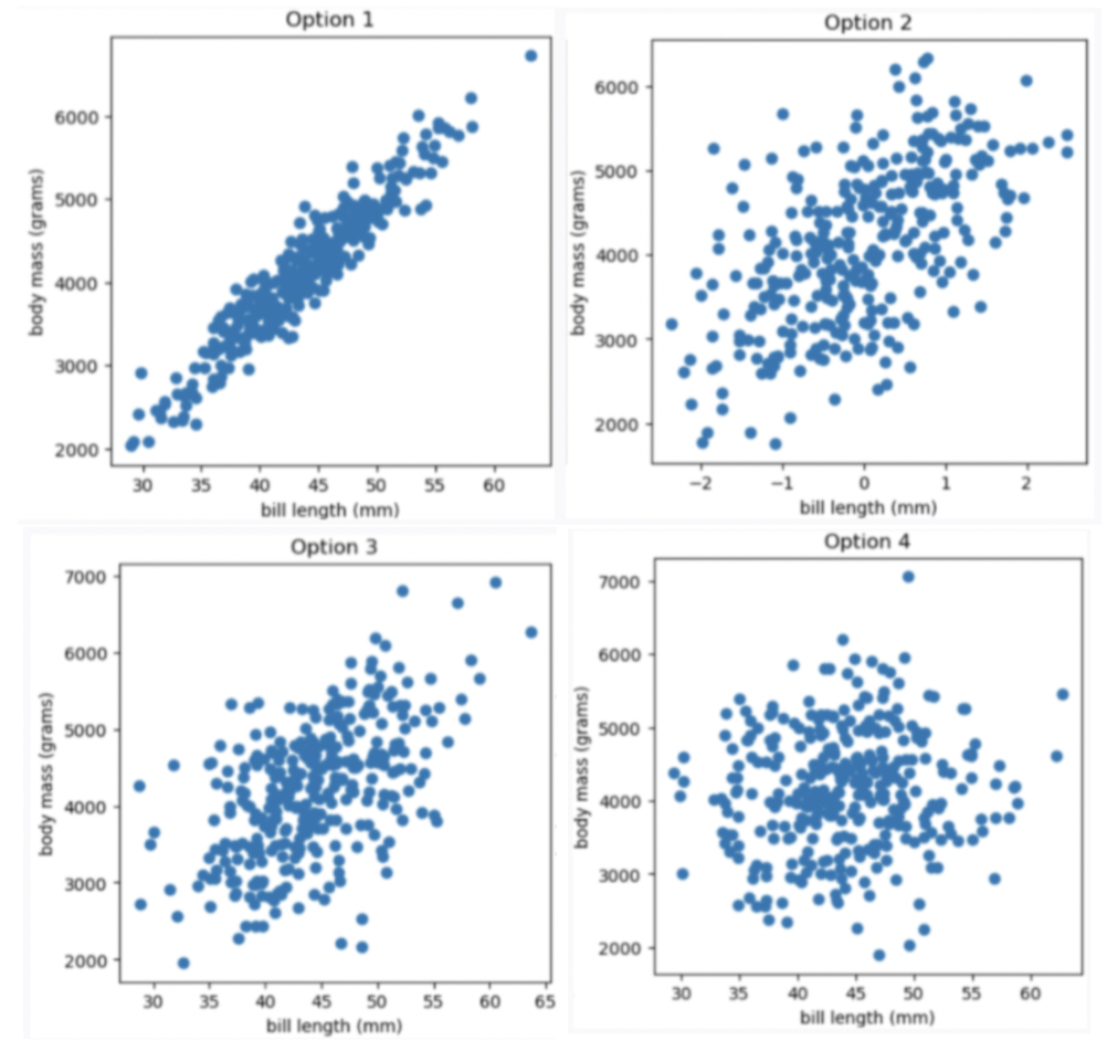
Let’s study the relationship between a penguin’s bill length (in millimeters) and mass (in grams). Suppose we’re given that
Which of the four scatter plots below describe the relationship between bill length and body mass, based on the information provided in the question?
Option 1
Option 2
Option 3
Option 4
Answer Option 3
Given the correlation coefficient is 0.55, bill length and body mass has a moderate positive correlation. We eliminate Option 1 (strong correlation) and Option 4 (weak correlation).
Given the average bill length is 44 mm, we expect our x-axis to have 44 at the middle, so we eliminate Option 2
The average score on this problem was 91%.
Suppose we want to find the regression line that uses bill length, x, to predict body mass, y. The line is of the form y = mx +\ b. What are m and b?
What is m? Give your answer as a number without any units, rounded to three decimal places.
What is b? Give your answer as a number without units, rounded to three decimal places.
Answer: m = 77, b = 812
m = r \cdot \frac{\text{SD of }y }{\text{SD of }x} = 0.55 \cdot \frac{840}{6} = 77 b = \text{mean of }y - m \cdot \text{mean of }x = 4200-77 \cdot 44 = 812
The average score on this problem was 92%.
What is the predicted body mass (in grams) of a penguin whose bill length is 44 mm? Give your answer as a number without any units, rounded to three decimal places.
Answer: 4200
y = mx\ +\ b = 77 \cdot 44 + 812 = 3388 +812 = 4200
The average score on this problem was 95%.
A particular penguin had a predicted body mass of 6800 grams. What is that penguin’s bill length (in mm)? Give your answer as a number without any units, rounded to three decimal places.
Answer: 77.766
In this question, we want to compute x value given y value y = mx\ +\ b y - b = mx \frac{y - b}{m} = x\ \ \text{(m is nonzero)} x = \frac{y - b}{m} = \frac{6800 - 812}{77} = \frac{5988}{77} \approx 77.766
The average score on this problem was 88%.
Below is the residual plot for our regression line.
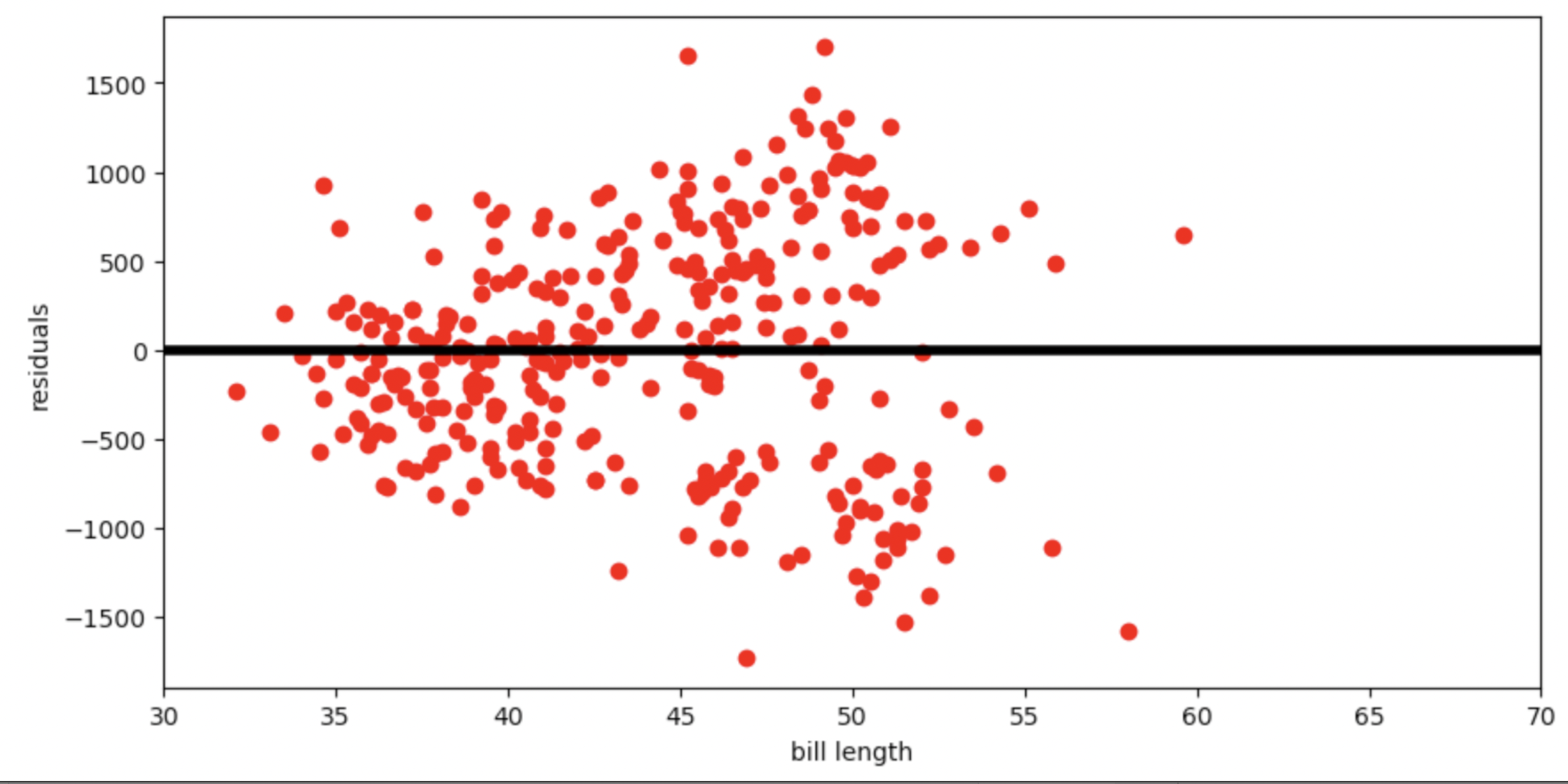
Which of the following is a valid conclusion that we can draw solely from the residual plot above?
For this dataset, there is another line with a lower root mean squared error
The root mean squared error of the regression line is 0
The accuracy of the regression line’s predictions depends on bill length
The relationship between bill length and body mass is likely non-linear
None of the above
Answer: The accuracy of the regression line’s predictions depends on bill length
The vertical spread in this residual plot is uneven, which implies that the regression line’s predictions aren’t equally accurate for all inputs. This doesn’t necessarily mean that fitting a nonlinear curve would be better. It just impacts how we interpret the regression line’s predictions.
The average score on this problem was 40%.
Suppose the price of an IKEA product and the cost to have it assembled are linearly associated with a correlation of 0.8. Product prices have a mean of 140 dollars and a standard deviation of 40 dollars. Assembly costs have a mean of 80 dollars and a standard deviation of 10 dollars. We want to predict the assembly cost of a product based on its price using linear regression.
The NORDMELA 4-drawer dresser sells for 200 dollars. How much do we predict its assembly cost to be?
Answer: 92 dollars
We first use the formulas for the slope, m, and intercept, b, of the regression line to find the equation. For our application, x is the price and y is the assembly cost since we want to predict the assembly cost based on price.
\begin{aligned} m &= r*\frac{\text{SD of }y}{\text{SD of }x} \\ &= 0.8*\frac{10}{40} \\ &= 0.2\\ b &= \text{mean of }y - m*\text{mean of }x \\ &= 80 - 0.2*140 \\ &= 80 - 28 \\ &= 52 \end{aligned}
Now we know the formula of the regression line and we simply plug in x=200 to find the associated y value.
\begin{aligned} y &= mx+b \\ y &= 0.2x+52 \\ &= 0.2*200+52 \\ &= 92 \end{aligned}
The average score on this problem was 76%.
The IDANÄS wardrobe sells for 80 dollars more than the KLIPPAN loveseat, so we expect the IDANÄS wardrobe will have a greater assembly cost than the KLIPPAN loveseat. How much do we predict the difference in assembly costs to be?
Answer: 16 dollars
The slope of a line describes the change in y for each change of 1 in x. The difference in x values for these two products is 80, so the difference in y values is m*80 = 0.2*80 = 16 dollars.
An equivalent way to state this is:
\begin{aligned} m &= \frac{\text{ rise, or change in } y}{\text{ run, or change in } x} \\ 0.2 &= \frac{\text{ rise, or change in } y}{80} \\ 0.2*80 &= \text{ rise, or change in } y \\ 16 &= \text{ rise, or change in } y \end{aligned}
The average score on this problem was 65%.
If we create a 95% prediction interval for the assembly cost of a 100 dollar product and another 95% prediction interval for the assembly cost of a 120 dollar product, which prediction interval will be wider?
The one for the 100 dollar product.
The one for the 120 dollar product.
Answer: The one for the 100 dollar product.
Prediction intervals get wider the further we get from the point (\text{mean of } x, \text{mean of } y) since all regression lines must go through this point. Since the average product price is 140 dollars, the prediction interval will be wider for the 100 dollar product, since it’s the further of 100 and 120 from 140.
The average score on this problem was 45%.
In this question, we’ll explore the relationship between the ages and incomes of credit card applicants.
The credit card company that owns the data in apps,
BruinCard, has decided not to give us access to the entire
apps DataFrame, but instead just a sample of
apps called small_apps. We’ll start by using
the information in small_apps to compute the regression
line that predicts the age of an applicant given their income.
For an applicant with an income that is \frac{8}{3} standard deviations above the
mean income, we predict their age to be \frac{4}{5} standard deviations above the
mean age. What is the correlation coefficient, r, between incomes and ages in
small_apps? Give your answer as a fully simplified
fraction.
Answer: r = \frac{3}{10}
To find the correlation coefficient r we use the equation of the regression line in standard units and solve for r as follows. \begin{align*} \text{predicted } y_{\text{(su)}} &= r \cdot x_{\text{(su)}} \\ \frac{4}{5} &= r \cdot \frac{8}{3} \\ r &= \frac{4}{5} \cdot \frac{3}{8} \\ r &= \frac{3}{10} \end{align*}
The average score on this problem was 52%.
Now, we want to predict the income of an applicant given their age.
We will again use the information in small_apps to find the
regression line. The regression line predicts that an applicant whose
age is \frac{4}{5} standard deviations
above the mean age has an income that is s standard deviations above the mean income.
What is the value of s? Give your
answer as a fully simplified fraction.
Answer: s = \frac{6}{25}
We again use the equation of the regression line in standard units, with the value of r we found in the previous part. \begin{align*} \text{predicted } y_{\text{(su)}} &= r \cdot x_{\text{(su)}} \\ s &= \frac{3}{10} \cdot \frac{4}{5} \\ s &= \frac{6}{25} \end{align*}
Notice that when we predict income based on age, our predictions are different than when we predict age based on income. That is, the answer to this question is not \frac{8}{3}. We can think of this phenomenon as a consequence of regression to the mean which means that the predicted variable is always closer to average than the original variable. In part (a), we start with an income of \frac{8}{3} standard units and predict an age of \frac{4}{5} standard units, which is closer to average than \frac{8}{3} standard units. Then in part (b), we start with an age of \frac{4}{5} and predict an income of \frac{6}{25} standard units, which is closer to average than \frac{4}{5} standard units. This happens because whenever we make a prediction, we multiply by r which is less than one in magnitude.
The average score on this problem was 21%.
BruinCard has now taken away our access to both apps and
small_apps, and has instead given us access to an even
smaller sample of apps called mini_apps. In
mini_apps, we know the following information:
We use the data in mini_apps to find the regression line
that will allow us to predict the income of an applicant given their
age. Just to test the limits of this regression line, we use it to
predict the income of an applicant who is -2 years old,
even though it doesn’t make sense for a person to have a negative
age.
Let I be the regression line’s prediction of this applicant’s income. Which of the following inequalities are guaranteed to be satisfied? Select all that apply.
I < 0
I < \text{mean income}
| I - \text{mean income}| \leq | \text{mean age} + 2 |
\dfrac{| I - \text{mean income}|}{\text{standard deviation of incomes}} \leq \dfrac{| \text{mean age} + 2 |}{\text{standard deviation of ages}}
None of the above.
Answer: I < \text{mean income}, \dfrac{| I - \text{mean income}|}{\text{standard deviation of incomes}} \leq \dfrac{| \text{mean age} + 2 |}{\text{standard deviation of ages}}
To understand this answer, we will investigate each option.
This option asks whether income is guaranteed to be negative. This is not necessarily true. For example, it’s possible that the slope of the regression line is 2 and the intercept is 10, in which case the income associated with a -2 year old would be 6, which is positive.
This option asks whether the predicted income is guaranteed to be lower than the mean income. It helps to think in standard units. In standard units, the regression line goes through the point (0, 0) and has slope r, which we are told is positive. This means that for a below-average x, the predicted y is also below average. So this statement must be true.
First, notice that | \text{mean age} + 2 | = | -2 - \text{mean age}|, which represents the horizontal distance betweeen these two points on the regression line: (\text{mean age}, \text{mean income}), (-2, I). Likewise, | I - \text{mean income}| represents the vertical distance between those same two points. So the inequality can be interpreted as a question of whether the rise of the regression line is less than or equal to the run, or whether the slope is at most 1. That’s not guaranteed when we’re working in original units, as we are here, so this option is not necessarily true.
Since standard deviation cannot be negative, we have \dfrac{| I - \text{mean income}|}{\text{standard deviation of incomes}} = \left| \dfrac{I - \text{mean income}}{\text{standard deviation of incomes}} \right| = I_{\text{(su)}}. Similarly, \dfrac{|\text{mean age} + 2|}{\text{standard deviation of ages}} = \left| \dfrac{-2 - \text{mean age}}{\text{standard deviation of ages}} \right| = -2_{\text{(su)}}. So this option is asking about whether the predicted income, in standard units, is guaranteed to be less (in absolute value) than the age. Since we make predictions in standard units using the equation of the regression line \text{predicted } y_{\text{(su)}} = r \cdot x_{\text{(su)}} and we know |r|\leq 1, this means |\text{predicted } y_{\text{(su)}}| \leq | x_{\text{(su)}}|. Applying this to ages (x) and incomes (y), this says exactly what the given inequality says. This is the phenomenon we call regression to the mean.
The average score on this problem was 69%.
Yet again, BruinCard, the company that gave us access to
apps, small_apps, and mini_apps,
has revoked our access to those three DataFrames and instead has given
us micro_apps, an even smaller sample of
apps.
Using micro_apps, we are again interested in finding the
regression line that will allow us to predict the income of an applicant
given their age. We are given the following information:
Suppose the standard deviation of incomes in micro_apps
is an integer multiple of the standard deviation of ages in
micro_apps. That is,
\text{standard deviation of income} = k \cdot \text{standard deviation of age}.
What is the value of k? Give your answer as an integer.
Answer: k = 4
To find this answer, we’ll use the definition of the regression line in original units, which is \text{predicted } y = mx+b, where m = r \cdot \frac{\text{SD of } y}{\text{SD of }x}, \: \: b = \text{mean of } y - m \cdot \text{mean of } x
Next we substitute these value for m and b into \text{predicted } y = mx + b, interpret x as age and y as income, and use the given information to find k. \begin{align*} \text{predicted } y &= mx+b \\ \text{predicted } y &= r \cdot \frac{\text{SD of } y}{\text{SD of }x} \cdot x+ \text{mean of } y - r \cdot \frac{\text{SD of } y}{\text{SD of }x} \cdot \text{mean of } x\\ \text{predicted income}&= r \cdot \frac{\text{SD of income}}{\text{SD of age}} \cdot \text{age}+ \text{mean income} - r \cdot \frac{\text{SD of income}}{\text{SD of age}} \cdot \text{mean age} \\ \frac{31}{2}&= -\frac{1}{3} \cdot k \cdot 24+ \frac{7}{2} + \frac{1}{3} \cdot k \cdot 33 \\ \frac{31}{2}&= -8k+ \frac{7}{2} + 11k \\ \frac{31}{2}&= 3k+ \frac{7}{2} \\ 3k &= \frac{31}{2} - \frac{7}{2} \\ 3k &= 12 \\ k &= 4 \end{align*}
Another way to solve this problem uses the equation of the regression line in standard units and the definition of standard units.
\begin{align*} \text{predicted } y_{\text{(su)}} &= r \cdot x_{\text{(su)}} \\ \frac{\text{predicted income} - \text{mean income}}{\text{SD of income}} &= r \cdot \frac{\text{age} - \text{mean age}}{\text{SD of age}} \\ \frac{\frac{31}{2} - \frac{7}{2}}{k\cdot \text{SD of age}} &= -\frac{1}{3} \cdot \frac{24 - 33}{\text{SD of age}} \\ \frac{12}{k\cdot \text{SD of age}} &= -\frac{1}{3} \cdot \frac{-9}{\text{SD of age}} \\ \frac{12}{k\cdot \text{SD of age}} &= \frac{3}{\text{SD of age}} \\ \frac{k\cdot \text{SD of age}}{\text{SD of age}} &= \frac{12}{3}\\ k &= 4 \end{align*}
The average score on this problem was 45%.
Raine is helping settle a debate between two friends on the
“superior" season — winter or summer. In doing so, they try to
understand the relationship between the number of sunshine hours per
month in January and the number of sunshine hours per month in July
across all cities in California in sun.
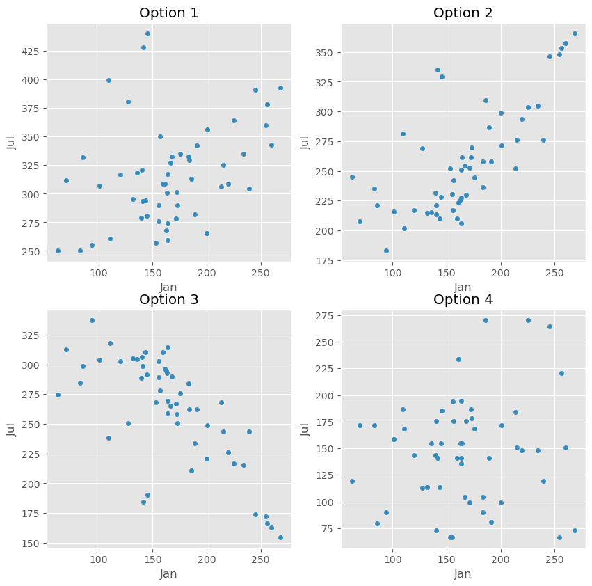
Raine finds the regression line that predicts the number of sunshine hours in July (y) for a city given its number of sunshine hours in January (x). In doing so, they find that the correlation between the two variables is \frac{2}{5}.
Which of these could be a scatter plot of number of sunshine hours in July vs. number of sunshine hours in January?
Option 1
Option 2
Option 3
Option 4
Answer: Option 1
Since r = \frac{2}{5}, the correct option must be a scatter plot with a mild positive (up and to the right) linear association. Option 3 can be ruled out immediately, since the linear association in it is negative (down and to the right). Option 2’s linear association is too strong for r = \frac{2}{5}, and Option 4’s linear association is too weak for r = \frac{2}{5}, which leaves Option 1.
The average score on this problem was 57%.
Suppose the standard deviation of the number of sunshine hours in January for cities in California is equal to the standard deviation of the number of sunshine hours in July for cities in California.
Raine’s hometown of Santa Clarita saw 60 more sunshine hours in January than the average California city did. How many more sunshine hours than average does the regression line predict that Santa Clarita will have in July? Give your answer as a positive integer. (Hint: You’ll need to use the fact that the correlation between the two variables is \frac{2}{5}.)
Answer: 24
At a high level, we’ll start with the formula for the regression line in standard units, and re-write it in a form that will allow us to use the information provided to us in the question.
Recall, the regression line in standard units is
\text{predicted }y_{\text{(su)}} = r \cdot x_{\text{(su)}}
Using the definitions of \text{predicted }y_{\text{(su)}} and x_{\text{(su)}} gives us
\frac{\text{predicted } y - \text{mean of }y}{\text{SD of }y} = r \cdot \frac{x - \text{mean of }x}{\text{SD of }x}
Here, the x variable is sunshine hours in January and the y variable is sunshine hours in July. Given that the standard deviation of January and July sunshine hours are equal, we can simplifies our formula to
\text{predicted } y - \text{mean of }y = r \cdot (x - \text{mean of }x)
Since we’re asked how much more sunshine Santa Clarita will have in July compared to the average, we’re interested in the difference y - \text{mean of} y. We were given that Santa Clarita had 60 more sunshine hours in January than the average, and that the correlation between the two variables(correlation coefficient) is \frac{2}{5}. In terms of the variables above, then, we know:
x - \text{mean of }x = 60.
r = \frac{2}{5}.
Then,
\text{predicted } y - \text{mean of }y = r \cdot (x - \text{mean of }x) = \frac{2}{5} \cdot 60 = 24
Therefore, the regression line predicts that Santa Clarita will have 24 more sunshine hours than the average California city in July.
The average score on this problem was 68%.
As we know, San Diego was particularly cloudy this May. More generally, Anthony, another California native, feels that California is getting cloudier and cloudier overall.
To imagine what the dataset may look like in a few years, Anthony subtracts 5 from the number of sunshine hours in both January and July for all California cities in the dataset – i.e., he subtracts 5 from each x value and 5 from each y value in the dataset. He then creates a regression line to use the new xs to predict the new ys.
What is the slope of Anthony’s new regression line?
Answer: \frac{2}{5}
To determine the slope of Anthony’s new regression line, we need to understand how the modifications he made to the dataset (subtracting 5 hours from each x and y value) affect the slope. In simple linear regression, the slope of the regression line (m in y = mx + b) is calculated using the formula:
m = r \cdot \frac{\text{SD of y}}{\text{SD of x}}
r, the correlation coefficient between the two variables, remains unchanged in Anthony’s modifications. Remember, the correlation coefficient is the mean of the product of the x values and y values when both are measured in standard units; by subtracting the same constant amount from each x value, we aren’t changing what the x values convert to in standard units. If you’re not convinced, convert the following two arrays in Python to standard units; you’ll see that the results are the same.
x1 = np.array([5, 8, 4, 2, 9])
x2 = x1 - 5
Furthermore, Anthony’s modifications also don’t change the standard deviations of the x values or y values, since the xs and ys aren’t any more or less spread out after being shifted “down” by 5. So, since r, \text{SD of }y, and \text{SD of }x are all unchanged, the slope of the new regression line is the same as the slope of the old regression line, pre-modification!
Given the fact that the correlation coefficient is \frac{2}{5} and the standard deviation of sunshine hours in January (\text{SD of }x) is equal to the standard deviation of sunshine hours in July (\text{SD of }y), we have
m = r \cdot \frac{\text{SD of }y}{\text{SD of }x} = \frac{2}{5} \cdot 1 = \frac{2}{5}
The average score on this problem was 73%.
Suppose the intercept of Raine’s original regression line – that is, before Anthony subtracted 5 from each x and each y – was 10. What is the intercept of Anthony’s new regression line?
-7
-5
-3
0
3
5
7
Answer: 7
Let’s denote the original intercept as b and the new intercept in the new dataset as b'. The equation for the original regression line is y = mx + b, where:
When Anthony subtracts 5 from each x and y value, the new regression line becomes y - 5 = m \cdot (x - 5) + b'
Expanding and rearrange this equation, we have
y = mx - 5m + 5 + b'
Remember, x and y here represent the number of sunshine hours in January and July, respectively, before Anthony subtracted 5 from each number of hours. This means that the equation for y above is equivalent to y = mx + b. Comparing, we see that
-5m + 5 + b' = b
Since m = \frac{2}{5} (from the previous part) and b = 10, we have
-5 \cdot \frac{2}{5} + 5 + b' = 10 \implies b' = 10 - 5 + 2 = 7
Therefore, the intercept of Anthony’s new regression line is 7.
The average score on this problem was 34%.
games contains information
about a sample of popular games. Besides other columns, there is a
column "Complexity" that contains the average complexity of
the game, a column "Rating" that contains the average
rating of the game, and a column "Play Time" that contains
the average play time of the game. We use the regression line to predict a game’s "Rating"
based on its "Complexity". We find that for the game
Wingspan, which has a "Complexity" that is 2
points higher than the average, the predicted "Rating" is 3
points higher than the average.
What can you conclude about the correlation coefficient r?
r < 0
r = 0
r > 0
We cannot make any conclusions about the value of r based on this information alone.
Answer: r > 0
To answer this problem, it’s useful to recall the regression line in standard units:
\text{predicted } y_{\text{(su)}} = r \cdot x_{\text{(su)}}
If a value is positive in standard units, it means that it is above
the average of the distribution that it came from, and if a value is
negative in standard units, it means that it is below the average of the
distribution that it came from. Since we’re told that Wingspan
has a "Complexity" that is 2 points higher than the
average, we know that x_{\text{(su)}}
is positive. Since we’re told that the predicted "Rating"
is 3 points higher than the average, we know that \text{predicted } y_{\text{(su)}} must also
be positive. As a result, r must also
be positive, since you can’t multiply a positive number (x_{\text{(su)}}) by a negative number and end
up with another positive number.
The average score on this problem was 74%.
What can you conclude about the standard deviations of “Complexity” and “Rating”?
SD of "Complexity" < SD of "Rating"
SD of "Complexity" = SD of "Rating"
SD of "Complexity" > SD of "Rating"
We cannot make any conclusions about the relationship between these two standard deviations based on this information alone.
Answer: SD of "Complexity" < SD of
"Rating"
Since the distance of the predicted "Rating" from its
average is larger than the distance of the "Complexity"
from its average, it might be reasonable to guess that the values in the
"Rating" column are more spread out. This is true, but
let’s see concretely why that’s the case.
Let’s start with the equation of the regression line in standard
units from the previous subpart. Remember that here, x refers to "Complexity" and
y refers to "Rating".
\text{predicted } y_{\text{(su)}} = r \cdot x_{\text{(su)}}
We know that to convert a value to standard units, we subtract the value by the mean of the column it came from, and divide by the standard deviation of the column it came from. As such, x_{\text{(su)}} = \frac{x - \text{mean of } x}{\text{SD of } x}. We can substitute this relationship in the regression line above, which gives us
\frac{\text{predicted } y - \text{mean of } y}{\text{SD of } y} = r \cdot \frac{x - \text{mean of } x}{\text{SD of } x}
To simplify things, let’s use what we were told. We were told that
the predicted "Rating" was 3 points higher than average.
This means that the numerator of the left side, \text{predicted } y - \text{mean of } y, is
equal to 3. Similarly, we were told that the "Complexity"
was 2 points higher than average, so x -
\text{mean of } x is 2. Then, we have:
\frac{3}{\text{SD of } y} = \frac{2r}{\text{SD of }x}
Note that for convenience, we included r in the numerator on the right-hand side.
Remember that our goal is to compare the SD of "Rating"
(y) to the SD of
"Complexity" (x). We now
have an equation that relates these two quantities! Since they’re both
currently on the denominator, which can be tricky to work with, let’s
take the reciprocal (i.e. “flip”) both fractions.
\frac{\text{SD of } y}{3} = \frac{\text{SD of }x}{2r}
Now, re-arranging gives us
\text{SD of } y \cdot \frac{2r}{3} = \text{SD of }x
Since we know that r is somewhere
between 0 and 1, we know that \frac{2r}{3} is somewhere between 0 and \frac{2}{3}. This means that \text{SD of } x is somewhere between 0 and
two-thirds of the value of \text{SD of }
y, which means that no matter what, \text{SD of } x < \text{SD of } y.
Remembering again that here "Complexity" is our x and "Rating" is our y, we have that the SD of
"Complexity" is less than the SD of
"Rating".
The average score on this problem was 42%.
Suppose that for children’s games, "Play Time" and
"Rating" are negatively linearly associated due to children
having short attention spans. Suppose that for children’s games, the
standard deviation of "Play Time" is twice the standard
deviation of "Rating", and the average
"Play Time" is 10 minutes. We use linear regression to
predict the "Rating" of a children’s game based on its
"Play Time". The regression line predicts that Don’t
Break the Ice, a children’s game with a "Play Time" of
8 minutes will have a "Rating" of 4. Which of the following
could be the average "Rating" for children’s games?
2
2.8
3.1
4
Answer: 3.1
Let’s recall the formulas for the regression line in original units,
since we’re given information in original units in this question (such
as the fact that for a "Play Time" of 8
minutes, the predicted "Rating" is 4
stars). Remember that throughout this question, "Play Time"
is our x and "Rating" is
our y.
The regression line is of the form y = mx + b, where
m = r \cdot \frac{\text{SD of } y}{\text{SD of }x}, b = \text{mean of }y - m \cdot \text{mean of } x
There’s a lot of information provided to us in the question – let’s think about what it means in the context of our xs and ys.
Given all of this information, we need to find possible values for the \text{mean of } y. Substituting our known values for m and b into y = mx + b gives us
y = \frac{r}{2} x + \text{mean of }y - 5r
Now, using the fact that if if x = 8, the predicted y is 4, we have
\begin{align*}4 &= \frac{r}{2} \cdot 8 + \text{mean of }y - 5r\\4 &= 4r - 5r + \text{mean of }y\\ 4 + r &= \text{mean of} y\end{align*}
Cool! We now know that the \text{mean of } y is 4 + r. We know that r must satisfy the relationship -1 \leq r < 0. By adding 4 to all pieces of this inequality, we have that 3 \leq r + 4 < 4, which means that 3 \leq \text{mean of } y < 4. Of the four options provided, only one is greater than or equal to 3 and less than 4, which is 3.1.
The average score on this problem was 55%.
df. The index of df contains the dog breed
names as str values. Besides other columns, there is a
column 'weight' (float) that contains typical weight (kg)
and a column 'height' (float) that contains typical height
(cm). He first runs the following code:
x = df.get('weight')
y = df.get('height')

def su(vals):
return (vals - vals.mean()) / np.std(vals)Select all of the Python snippets that correctly compute the
correlation coefficient into the variable r.
Snippet 1:
r = (su(x) * su(y)).mean()Snippet 2:
r = su(x * y).mean()Snippet 3:
t = 0
for i in range(len(x)):
    t = t + su(x[i]) * su(y[i])
r = t / len(x)
Snippet 4:
t = np.array([])
for i in range(len(x)):
    t = np.append(t, su(x)[i] * su(y)[i])
r = t.mean()
Snippet 1
Snippet 2
Snippet 3
Snippet 4
Answer: Snippet 1 & 4
Snippet 1: Recall from the reference sheet, the correlation
coefficient is r = (su(x) * su(y)).mean().
Snippet 2: We have to standardize each variable separately so this snippet doesn’t work.
Snippet 3: Note that for this snippet we’re standardizing each
data point within each variable separately, and so we’re not really
standardizing the entire variable correctly. In other words, applying
su(x[i]) to a singular data point is just going to convert
this data point to zero, since we’re only inputting one data point into
su().
Snippet 4: Note that this code is just the same as Snippet 1, except we’re now directly computing the product of each corresponding data points individually. Hence this Snippet works.
The average score on this problem was 81%.
Sam computes the following statistics for his sample:
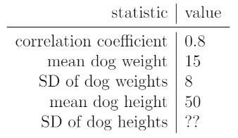
The best-fit line predicts that a dog with a weight of 10 kg has a height of 45 cm.
What is the SD of dog heights?
2
4.5
10
25
45
None of the above
Answer: Option 3: 10
The best fit line in original units are given by
y = mx + b where m = r * (SD of y) / (SD of x)
and b = (mean of y) - m * (mean of x) (refer to reference
sheet). Let c be the STD of y, which we’re trying to find,
then our best fit line is now y = (0.8*c/8)x +
(50-(0.8*c/8)*15). Plugging the two values they gave us into our
best fit line and simplifying gives 45 =
0.1*c*10 + (50 - 1.5*c) which simplifies to 45 = 50 - 0.5*c which gives us an answer of
c = 10.
The average score on this problem was 89%.
Assume that the statistics in part b) still hold. Select all of the statements below that are true. (You don’t need to finish part b) in order to solve this question.)
The relationship between dog weight and height is linear.
The root mean squared error of the best-fit line is smaller than 5.
The best-fit line predicts that a dog that weighs 15 kg will be 50 cm tall.
The best-fit line predicts that a dog that weighs 10 kg will be shorter than 50 cm.
Answer: Option 3 & 4
Option 1: We cannot determine whether two variables are linear simply from a line of best fit. The line of best fit just happens to find the best linear relationship between two varaibles, not whether or not the variables have a linear relationship.
Option 2: To calculate the root mean squared error, we need the actual data points so we can calculate residual values. Seeing that we don’t have access to the data points, we cannot say that the root mean squared error of the best-fit line is smaller than 5.
Option 3: This is true accrding to the problem statement given in part b
Option 4: This is true since we expect there to be a positive correlation between dog height and weight. So dogs that are lighter will also most likely be shorter. (ie a dog that is lighter than 15 kg will most likely be shorter than 50cm)
The average score on this problem was 72%.
Are nonfiction books longer than fiction books?
Choose the best data science tool to help you answer this question.
hypothesis testing
permutation (A/B) testing
Central Limit Theorem
regression
Answer: permutation (A/B) testing
The question Are nonfiction books longer than fiction books? is investigating the difference between two underlying populations (nonfiction books and fiction books). A permutation test is the best data science tool when investigating differences between two underlying distributions.
The average score on this problem was 90%.
Do people have more friends as they get older?
Choose the best data science tool to help you answer this question.
hypothesis testing
permutation (A/B) testing
Central Limit Theorem
regression
Answer: regression
The question at hand is investigating two continuous variables (time and number of friends). Regression is the best data science tool as it is dealing with two continuous variables and we can understand correlations between time and the number of friends.
The average score on this problem was 90%.
Does an ice cream shop sell more chocolate or vanilla ice cream cones?
Choose the best data science tool to help you answer this question.
hypothesis testing
permutation (A/B) testing
Central Limit Theorem
regression
Answer: hypothesis testing
The question at hand is dealing with differences between sales of different flavors of ice cream, which is the same thing as the total of ice cream cones sold. We can use hypothesis testing to test our null hypothesis that the count of Vanilla cones sold is higher than Chocolate, and our alternative hypothesis that the count of Chocolate cones sold is more than Vanilla. A permutation test is not suitable here because we are not comparing any numerical quantity associated with each group. A permutation test could be used to answer questions like “Are chocolate ice cream cones more expensive than vanilla ice cream cones?” or “Do chocolate ice cream cones have more calories than vanilla ice cream cones?”, or any other question where you are tracking a number (cost or calories) along with each ice cream cone. In our case, however, we are not tracking a number along with each individual ice cream cone, but instead tracking a total of ice cream cones sold.
An analogy to this hypothesis test can be found in the “fair or unfair coin” problem in Lectures 20 and 21, where our null hypothesis is that the coin is fair and our alternative hypothesis is that the coin is unfair. The “fairness” of the coin is not a numerical quantity that we can track with each individual coin flip, just like how the count of ice cream cones sold is not a numerical quantity that we can track with each individual ice cream cone.
The average score on this problem was 57%.