← return to practice.dsc10.com
Instructor(s): Janine Tiefenbruck, Suraj Rampure
This exam was administered remotely via Gradescope. The exam was open-internet, and students were able to use Jupyter Notebooks. They had 3 hours to work on it.
Note (groupby / pandas 2.0): Pandas 2.0+ no longer
silently drops columns that can’t be aggregated after a
groupby, so code written for older pandas may behave
differently or raise errors. In these practice materials we use
.get() to select the column(s) we want after
.groupby(...).mean() (or other aggregations) so that our
solutions run on current pandas. On real exams you will not be penalized
for omitting .get() when the old behavior would have
produced the same answer.
Welcome to the Final Exam! In honor of the (at the time) brand-new Comic-Con Museum that just opened at Balboa Park here in San Diego, this exam will contain questions about various museums and zoos around the world.
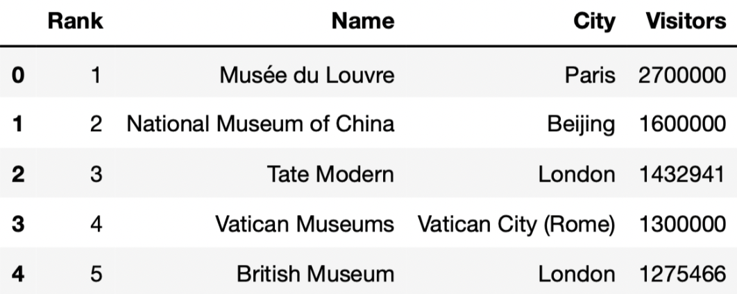
In this question, we’ll work with the DataFrame
art_museums, which contains the name, city, number of
visitors in 2019, and rank (based on number of visitors) for the 100
most visited art museums in 2019. The first few rows of
art_museums are shown below.
Tip: Open this page in another tab, so that it is easy to refer to this data description as you work through the exam.
Which of the following blocks of code correctly assigns
random_art_museums to an array of the names of 10 art
museums, randomly selected without replacement from those in
art_museums? Select all that apply.
Option 1:
def get_10(df):
    return np.array(df.sample(10).get('Name'))

random_art_museums = get_10(art_museums)
Option 2:
def get_10(art_museums):
    return np.array(art_museums.sample(10).get('Name'))

random_art_museums = get_10(art_museums)
Option 3:
def get_10(art_museums):
    random_art_museums = np.array(art_museums.sample(10).get('Name'))

random_art_museums = get_10(art_museums)
Option 4:
def get_10():
    return np.array(art_museums.sample(10).get('Name'))

random_art_museums = get_10()
Option 5:
random_art_museums = np.array([])

def get_10():
    random_art_museums = np.array(art_museums.sample(10).get('Name'))
    return random_art_museums

get_10()
Option 1
Option 2
Option 3
Option 4
Option 5
None of the above
Answers: Option 1, Option 2, and Option 4
Note that if df is a DataFrame, then
df.sample(10) is a DataFrame containing 10 randomly
selected rows in df. With that in mind, let’s look at all
of our options.
get_10 takes in a DataFrame df and returns an
array containing 10 randomly selected values in df’s
'Name' column. After defining get_10, we
assign random_art_museums to the result of calling
get_10(art_museums). This assigns
random_art_museums as intended, so Option 1 is
correct.art_museums and Option 1 uses the parameter name
df (both in the def line and in the function
body); this does not change the behavior of get_10 or the
lines afterward.get_10 here does not return
anything! So, get_10(art_museums) evaluates to
None (which means “nothing” in Python), and
random_art_museums is also None, meaning
Option 3 is incorrect.get_10 does not take in any inputs. However,
the body of get_10 contains a reference to the DataFrame
art_museums, which is ultimately where we want to sample
from. As a result, get_10 does indeed return an array
containing 10 randomly selected museum names, and
random_art_museums = get_10() correctly assigns
random_art_museums to this array, so Option 4 is
correct.get_10 returns the
correct array. However, outside of the function,
random_art_museums is never assigned to the output of
get_10. (The variable name random_art_museums
inside the function has nothing to do with the array defined before and
outside the function.) As a result, after running the line
get_10() at the bottom of the code block,
random_art_museums is still an empty array, and as such,
Option 5 is incorrect.
The average score on this problem was 85%.
London has the most art museums in the top 100 of any city in the
world. The most visited art museum in London is
'Tate Modern'.
Which of the following blocks of code correctly assigns
best_in_london to 'Tate Modern'? Select all
that apply.
Option 1:
def most_common(df, col):
    return df.groupby(col).count().sort_values(by='Rank', ascending=False).index[0]

def most_visited(df, col, value):
    return df[df.get(col)==value].sort_values(by='Visitors', ascending=False).get('Name').iloc[0]

best_in_london = most_visited(art_museums, 'City', most_common(art_museums, 'City'))
Option 2:
def most_common(df, col):
    print(df.groupby(col).count().sort_values(by='Rank', ascending=False).index[0])

def most_visited(df, col, value):
    print(df[df.get(col)==value].sort_values(by='Visitors', ascending=False).get('Name').iloc[0])

best_in_london = most_visited(art_museums, 'City', most_common(art_museums, 'City'))
Option 3:
def most_common(df, col):
    return df.groupby(col).count().sort_values(by='Rank', ascending=False).index[0]

def most_visited(df, col, value):
    print(df[df.get(col)==value].sort_values(by='Visitors', ascending=False).get('Name').iloc[0])

best_in_london = most_visited(art_museums, 'City', most_common(art_museums, 'City'))
Option 1
Option 2
Option 3
None of the above
Answer: Option 1 only
At a glance, it may seem like there’s a lot of reading to do to
answer the question. However, it turns out that all 3 options follow
similar logic; the difference is in their use of print and
return statements. Whenever we want to “save” the output of
a function to a variable name or use it in another function, we need to
return somewhere within our function. Only Option 1
contains a return statement in both
most_common and most_visited, so it is the
only correct option.
Let’s walk through the logic of Option 1 (which we don’t necessarily need to do to answer the problem, but we should in order to enhance our understanding):
most_common to find the city with the
most art museums. most_common does this by grouping the
input DataFrame df (art_museums, in this case)
by 'City' and using the .count() method to
find the number of rows per 'City'. Note that when using
.count(), all columns in the aggregated DataFrame will
contain the same information, so it doesn’t matter which column you use
to extract the counts per group. After sorting by one of these columns
('Rank', in this case) in decreasing order,
most_common takes the first value in the
index, which will be the name of the 'City'
with the most art museums. This is London,
i.e. most_common(art_museums, 'City') evaluates to
'London' in Option 1 (in Option 2, it evaluates to
None, since most_common there doesn’t
return anything).most_visited to find the museum with the
most visitors in the city with the most museums. This is achieved by
keeping only the rows of the input DataFrame df (again,
art_museums in this case) where the value in the
col ('City') column is value
(most_common(art_museums, 'City'), or
'London'). Now that we only have information for museums in
London, we can sort by 'Visitors' to find the most visited
such museum, and take the first value from the resulting
'Name' column. While all 3 options follow this logic, only
Option 1 returns the desired value, and so only Option
1 assigns best_in_london correctly. (Even if Option 2’s
most_visited used return instead of
print, it still wouldn’t work, since Option 2’s
most_common also uses print instead of
return).
The average score on this problem was 86%.
In this question, we’ll keep working with the
art_museums DataFrame.
(Remember to keep the data description from the top of the exam open in another tab!)
'Tate Modern' is the most popular art museum in London.
But what’s the most popular art museum in each city?
It turns out that there’s no way to answer this easily using the
tools that you know about so far. To help, we’ve created a new Series
method, .last(). If s is a Series,
s.last() returns the last element of s
(i.e. the element at the very end of s).
.last() works with .groupby, too (just like
.mean() and .count()).
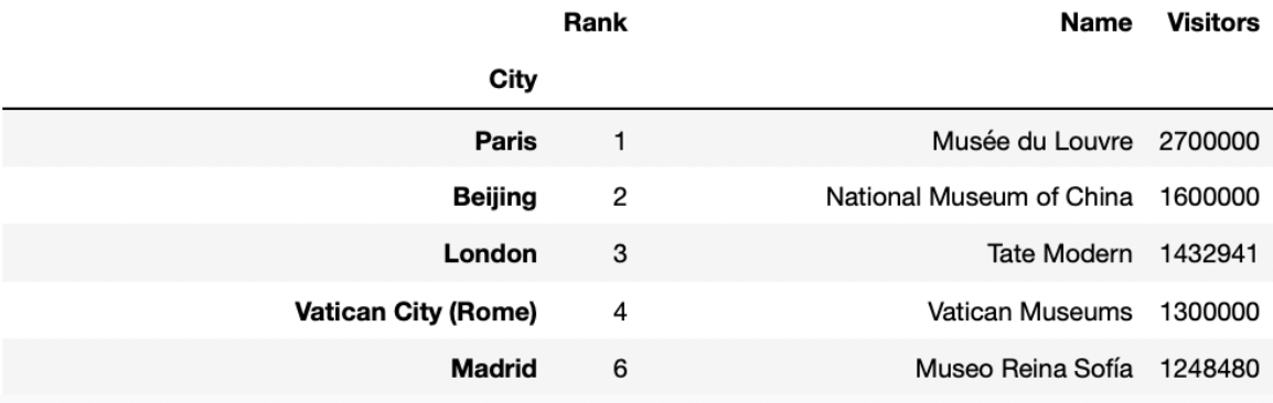
Fill in the blanks so that the code below correctly assigns
best_per_city to a DataFrame with one row per city, that
describes the name, number of visitors, and rank of the most visited art
museum in each city. best_per_city should be sorted in
decreasing order of number of visitors. The first few rows of
best_per_city are shown below.
best_per_city = __(a)__.groupby(__(b)__).last().__(c)__Answers:
art_museums.sort_values('Visitors', ascending=True)'City'sort_values('Visitors', ascending=False)Let’s take a look at the completed implementation.
best_per_city = art_museums.sort_values('Visitors', ascending=True).groupby('City').last().sort_values('Visitors', ascending=False)We first sort the row in art_museums by the number of
'Visitors' in ascending order. Then
groupby('City'), so that we have one row per city. Recall,
we need an aggregation method after using groupby(). In
this question, we use last() to only keep the one last row
for each city. Since in blank (a) we have sorted the rows by
'Visitors', so last() keeps the row that
contains the name of the most visited museum in that city. At last we
sort this new DataFrame by 'Visitors' in descending order
to fulfill the question’s requirement.
The average score on this problem was 65%.
Assume you’ve defined best_per_city correctly.
Which of the following options evaluates to the number of visitors to the most visited art museum in Amsterdam? Select all that apply.
best_per_city.get('Visitors').loc['Amsterdam']
best_per_city[best_per_city.index == 'Amsterdam'].get('Visitors').iloc[0]
best_per_city[best_per_city.index == 'Amsterdam'].get('Visitors').iloc[-1]
best_per_city[best_per_city.index == 'Amsterdam'].get('Visitors').loc['Amsterdam']
None of the above
Answer:
best_per_city.get('Visitors').loc['Amsterdam'],
best_per_city[best_per_city.index == 'Amsterdam'].get('Visitors').iloc[0],
best_per_city[best_per_city.index == 'Amsterdam'].get('Visitors').iloc[-1],
best_per_city[best_per_city.index == 'Amsterdam'].get('Visitors').loc['Amsterdam']
(Select all except “None of the above”)
best_per_city.get('Visitors').loc['Amsterdam'] We first
use .get(column_name) to get a series with number of
visitors to the most visited art museum, and then locate the number of
visitors to the most visited art museum in Amsterdam using
.loc[index] since we have "City" as index.
best_per_city[best_per_city.index == 'Amsterdam'].get('Visitors').iloc[0]
We first query the best_per_city to only include the
DataFrame with one row with index 'Amsterdam'. Then, we get
the 'Visitors' column of this DataFrame. Finally, we use
iloc[0] to access the first and the only value in this
column.
best_per_city[best_per_city.index == 'Amsterdam'].get('Visitors').iloc[-1]
We first query the best_per_city to only include the
DataFrame with one row with index 'Amsterdam'. Then, we get
the 'Visitors' column of this DataFrame. Finally, we use
iloc[-1] to access the last and the only value in this
column.
best_per_city[best_per_city.index == 'Amsterdam'].get('Visitors').loc['Amsterdam']
We first query the best_per_city to only include the
DataFrame with one row with index 'Amsterdam'. Then, we get
the 'Visitors' column of this DataFrame. Finally, we use
loc['Amsterdam'] to access the value in this column with
index 'Amsterdam'.
The average score on this problem was 84%.
The table below shows the average amount of revenue from different sources for art museums in 2003 and 2013.
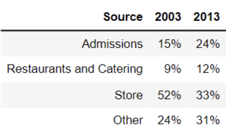
What is the total variation distance between the distribution of revenue sources in 2003 and the distribution of revenue sources in 2013? Give your answer as a proportion (i.e. a decimal between 0 and 1), not a percentage. Round your answer to three decimal places.
Answer: 0.19
Recall, the total variation distance (TVD) is the sum of the absolute differences in proportions, divided by 2. The absolute differences in proportions for each source are as follows:
Then, we have
\text{TVD} = \frac{1}{2} (0.09 + 0.03 + 0.19 + 0.07) = 0.19
The average score on this problem was 95%.
Which type of visualization would be best suited for comparing the two distributions in the table?
Scatter plot
Line plot
Overlaid histogram
Overlaid bar chart
Answer: Overlaid bar chart
A scatter plot visualizes the relationship between two numerical variables. In this problem, we only have to visualize the distribution of a categorical variable.
A line plot shows trends in numerical variables over time. In this problem, we only have categorical variables. Moreover, when it says over time, it is suitable for plotting change in multiple years (e.g. 2001, 2002, 2003, … , 2013), or even with data of days. In this question, we only want to compare the distribution of 2003 and 2013, this makes the line plot not useful. In addition, if you try to draw a line plot for this question, you will find the line plot fails to visualize distribution (e.g. the idea of 15%, 9%, 52%, and 24% add up to 100%).
An overlaid graph is useful in this question since this visualizes comparison between the two distributions.
However, an overlaid histogram is not useful in this problem. The key reason is the differences between a histogram and a bar chart.
Bar Chart: Space between the bars; 1 categorical axis, 1 numerical
axis; order does not matter
Histogram: No space between the bars; intervals on axis; 2 numerical
axes; order matters
In the question, we are plotting 2003 and 2013 distributions of four categories (Admissions, Restaurants and Catering, Store, and Other). Thus, an overlaid bar chart is more appropriate.
The average score on this problem was 74%.
Note: This problem is out of scope; it covers material no longer included in the course.
Notably, there was an economic recession in 2008-2009. Which of the following can we conclude was an effect of the recession?
The increase in revenue from admissions, as more people were visiting museums.
The decline in revenue from museum stores, as people had less money to spend.
The decline in total revenue, as fewer people were visiting museums.
None of the above
Answer: None of the above
Since we are only given the distribution of the revenue, and have no information about the amount of revenue in 2003 and 2013, we cannot conclude how the revenue has changed from 2003 to 2013 after the recession.
For instance, if the total revenue in 2003 was 100 billion USD and the total revenue in 2013 was 50 billion USD, revenue from admissions in 2003 was 100 * 15% = 15 billion USD, and revenue from admissions in 2003 was 50 * 24% = 12 billion USD. In this case, we will have 15 > 12, the revenue from admissions has declined rather than increased (As stated by ‘The increase in revenue from admissions, as more people were visiting museums.’). Similarly, since we don’t know the total revenue in 2003 and 2013, we cannot conclude ‘The decline in revenue from museum stores, as people had less money to spend.’ or ‘The decline in total revenue, as fewer people were visiting museums.’
The average score on this problem was 72%.
The Museum of Natural History has a large collection of dinosaur bones, and they know the approximate year each bone is from. They want to use this sample of dinosaur bones to estimate the total number of years that dinosaurs lived on Earth. We’ll make the assumption that the sample is a uniform random sample from the population of all dinosaur bones. Which statistic below will give the best estimate of the population parameter?
sample sum
sample max - sample min
2 \cdot (sample mean - sample min)
2 \cdot (sample max - sample mean)
2 \cdot sample mean
2 \cdot sample median
Answer: sample max - sample min
Our goal is to estimate the total number of years that dinosaurs lived on Earth. In other words, we want to know the range of time that dinosaurs lived on Earth, and by definition range = biggest value - smallest value. By using “sample max - sample min”, we calculate the difference between the earliest and the latest dinosaur bones in this uniform random sample, which helps us to estimate the population range.
The average score on this problem was 52%.
The curator at the Museum of Natural History, who happens to have taken a data science course in college, points out that the estimate of the parameter obtained from this sample could certainly have come out differently, if the museum had started with a different sample of bones. The curator suggests trying to understand the distribution of the sample statistic. Which of the following would be an appropriate way to create that distribution?
bootstrapping the original sample
using the Central Limit Theorem
both bootstrapping and the Central Limit Theorem
neither bootstrapping nor the Central Limit Theorem
Answer: neither bootstrapping nor the Central Limit Theorem
Recall, the Central Limit Theorem (CLT) says that the probability distribution of the sum or average of a large random sample drawn with replacement will be roughly normal, regardless of the distribution of the population from which the sample is drawn. Thus, the theorem only applies when our sample statistics is sum or average, while in this question, our statistics is range, so CLT does not apply.
Bootstrapping is a valid technique for estimating measures of central tendency, e.g. the population mean, median, standard deviation, etc. It doesn’t work well in estimating extreme or sensitive values, like the population maximum or minimum. Since the statistic we’re trying to estimate is the difference between the population maximum and population minimum, bootstrapping is not appropriate.
The average score on this problem was 20%.
Now, the Museum of Natural History wants to know how many visitors they have in a year. However, their computer systems are rather archaic and so they aren’t able to keep track of the number of tickets sold for an entire year. Instead, they randomly select five days in the year, and keep track of the number of visitors on those days. Let’s call these numbers v_1, v_2, v_3, v_4, and v_5.
Which of the following is the best estimate the number of visitors for the entire year?
v_1 + v_2 + v_3 + v_4 + v_5
\frac{5}{365}\cdot(v_1 + v_2 + v_3 + v_4 + v_5)
\frac{365}{5}\cdot(v_1 + v_2 + v_3 + v_4 + v_5)
365\cdot v_3
Answer: \frac{365}{5}\cdot(v_1 + v_2 + v_3 + v_4 + v_5)
Our sample is the number of visitors on the five days, and our population is the number of visitors in all 365 days.
First, we calculate the sample mean, the average number of visitors in the 5 days, which is m = \frac{1}{5}\cdot(v_1 + v_2 + v_3 + v_4 + v_5). We use this statistic to estimate the population mean, the average number of visitors in this year.
Then, we use the estimated population mean to calculate the estimated population sum, so we multiply the number of days in a year (365) with the estimated population mean. We get 365 m = \frac{365}{5}\cdot(v_1 + v_2 + v_3 + v_4 + v_5)
The average score on this problem was 92%.
Now we’re interested in predicting the admission cost of a museum based on its number of visitors. Suppose:
admission cost and number of visitors are linearly associated with a correlation coefficient of 0.25,
the number of visitors at the Museum of Natural History is six standard deviations below average,
the average cost of museum admission is 15 dollars, and
the standard deviation of admission cost is 3 dollars.
What would the regression line predict for the admission cost (in dollars) at the Museum of Natural History? Give your answer as a number without any units, rounded to three decimal places.
Answer: 10.500
Recall, we can make predictions in standard units with the following formula
\text{predicted}\ y_{su} = r \cdot x_{su}
We’re given that the correlation coefficient, r, between visitors and admission cost is 0.25. Here, we’re using the number of visitors (x) to predict admission cost (y). Given that the number of visitors at the Museum of Natural History is 6 standard deviations below average,
\text{predicted}\ y_{su} = r \cdot x_{su} = 0.25 \cdot -6 = -1.5
We then compute y, which is the admission cost (in dollars) at the Museum of Natural History.
\begin{align*} y_{su} &= \frac{y- \text{Mean of } y}{\text{SD of } y}\\ -1.5 &= \frac{y-15}{3} \\ -1.5 \cdot 3 &= y-15\\ -4.5 + 15 &= y\\ y &= \boxed{10.5} \end{align*}
So, the regression line predicts that the admission cost at the Museum of Natural History is $10.50.
The average score on this problem was 62%.
Researchers from the San Diego Zoo, located within Balboa Park, collected physical measurements of several species of penguins in a region of Antarctica.
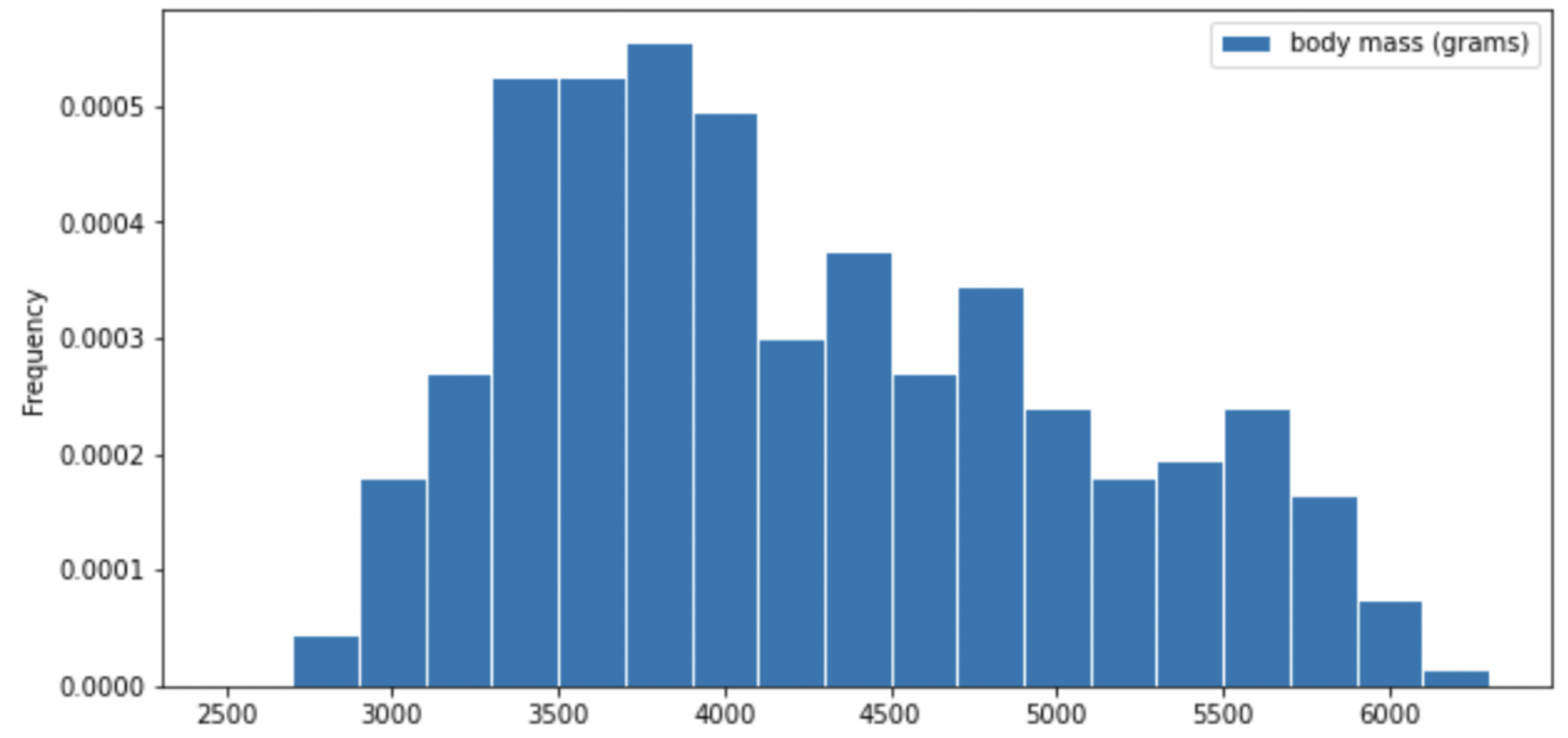
One piece of information they tracked for each of 330 penguins was its mass in grams. The average penguin mass is 4200 grams, and the standard deviation is 840 grams.
Consider the histogram of mass below.
Select the true statement below.
The median mass of penguins is larger than the average mass of penguins
The median mass of penguins is roughly equal to the average mass of penguins (within 50 grams)
The median mass of penguins is less than the average mass of penguins
It is impossible to determine the relationship between the median and average mass of penguins just by looking at the above histogram
Answer: The median mass of penguins is less than the average mass of penguins
This is a distribution that is skewed to the right, so mean is greater than median.
The average score on this problem was 87%.
Which of the following is a valid conclusion that we can draw solely from the histogram above?
The number of penguins with a mass of exactly 3500 grams is greater than the number of penguins with a mass of exactly 5500 grams.
The number of penguins with a mass of at most 3500 grams is greater than the number of penguins with a mass of at least 5500 grams.
There is an odd number of penguins in the dataset.
The number penguins with a mass of exactly 4000 grams is greater than zero.
None of the above.
Answer: The number of penguins with a mass of at most 3500 grams is greater than the number of penguins with a mass of at least 5500 grams.
Recall, a histogram has intervals on the axis, so we cannot know the frequency of an exact value. Thus, we cannot conclude statements 1, 3, 4. Since the frequency of an exact value is unknown, for statement 3, it is possible that all numbers we have in this distribution are even. Although in the graph, we are only given frequency rather than number, we can justify statement 2 by comparing the area in the left side of 3500, and the area in the right side of 5500. You can either estimate by visually comparing the areas of both parts or compute the area sum of both sides by estimating the bars’ height and windth.
The average score on this problem was 89%.
For your convenience, we show the histogram of mass again below.
Recall, there are 330 penguins in our dataset. Their average mass is 4200 grams, and the standard deviation of mass is 840 grams.
Per Chebyshev’s inequality, at least what percentage of penguins have a mass between 3276 grams and 5124 grams? Input your answer as a percentage between 0 and 100, without the % symbol. Round to three decimal places.
Answer: 17.355
Recall, Chebyshev’s inequality states that No matter what the shape of the distribution is, the proportion of values in the range “average ± z SDs” is at least 1 - \frac{1}{z^2}.
To approach the problem, we’ll start by converting 3276 grams and 5124 grams to standard units. Doing so yields \frac{3276 - 4200}{840} = -1.1, similarly, \frac{5124 - 4200}{840} = 1.1. This means that 3276 is 1.1 standard deviations below the mean, and 5124 is 1.1 standard deviations above the mean. Thus, we are calculating the proportion of values in the range “average ± 1.1 SDs”.
When z = 1.1, we have 1 - \frac{1}{z^2} = 1 - \frac{1}{1.1^2} \approx 0.173553719, which as a percentage rounded to three decimal places is 17.355\%.
The average score on this problem was 76%.
Per Chebyshev’s inequality, at least what percentage of penguins have a mass between 1680 grams and 5880 grams?
50%
55.5%
65.25%
68%
75%
88.8%
95%
Answer: 75%
Recall: proportion with z SDs of the mean
| Percent in Range | All Distributions (via Chebyshev’s Inequality) | Normal Distributions |
|---|---|---|
| \text{average} \pm 1 \ \text{SD} | \geq 0\% | \approx 68\% |
| \text{average} \pm 2\text{SDs} | \geq 75\% | \approx 95\% |
| \text{average} \pm 3\text{SDs} | \geq 88\% | \approx 99.73\% |
To approach the problem, we’ll start by converting 3276 grams and 5124 grams to standard units. Doing so yields \frac{1680 - 4200}{840} = -3, similarly, \frac{5880 - 4200}{840} = 2. This means that 1680 is 3 standard deviations below the mean, and 5880 is 2 standard deviations above the mean.
Proportion of values in [-3 SUs, 2 SUs] >= Proportion of values in [-2 SUs, 2 SUs] >= 75% (Since we cannot assume that the distribution is normal, we look at the All Distributions (via Chebyshev’s Inequality) column for proportion).
Thus, at least 75% of the penguins have a mass between 1680 grams and 5880 grams.
The average score on this problem was 72%.
The distribution of mass in grams is not roughly normal. Is the distribution of mass in standard units roughly normal?
Yes
No
Impossible to tell
Answer: No
The shape of the distribution does not change since we are scaling the x values for all data.
The average score on this problem was 60%.
Suppose all 330 penguin body masses (in grams) that the researchers
collected are stored in an array called masses. We’d like
to estimate the probability that two different randomly selected
penguins from our dataset have body masses within 50 grams of one
another (including a difference of exactly 50 grams). Fill in the
missing pieces of the simulation below so that the function
estimate_prob_within_50g returns an estimate for this
probability.
def estimate_prob_within_50g():
    num_reps = 10000
    within_50g_count = 0
    for i in np.arange(num_reps):
        two_penguins = np.random.choice(__(a)__)
        if __(b)__:
            within_50g_count = within_50g_count + 1
    return within_50g_count / num_reps
What goes in blank (a)? What goes in blank (b)?
Answer: (a) masses, 2, replace=False
(b) abs(two_penguins[0] - two_penguins[1])<=50
np.random.choice( ) can have three parameters
array, n, replace=False, and returns n elements from the
array at random, without replacement. We are randomly choosing 2
different penguins from the masses
array, so we are using np.random.choice( )
without replacement.two_penguins and
calculating their absolute difference with abs(). And in
this if condition, we only want to have penguins with
absolute difference less than or equal to 50, so we write a
<= condition to justify whether the generated pairs of
penguins fulfill this requirement.
The average score on this problem was 84%.
Recall, there are 330 penguins in our dataset. Their average mass is 4200 grams, and the standard deviation of mass is 840 grams. Assume that the 330 penguins in our dataset are a random sample from the population of all penguins in Antarctica. Our sample gives us one estimate of the population mean.
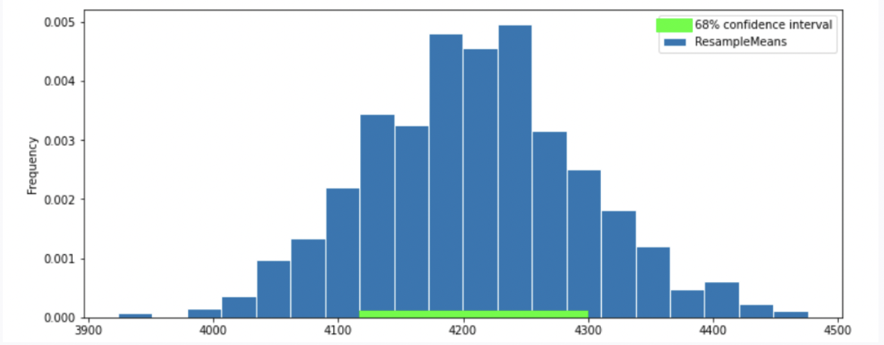
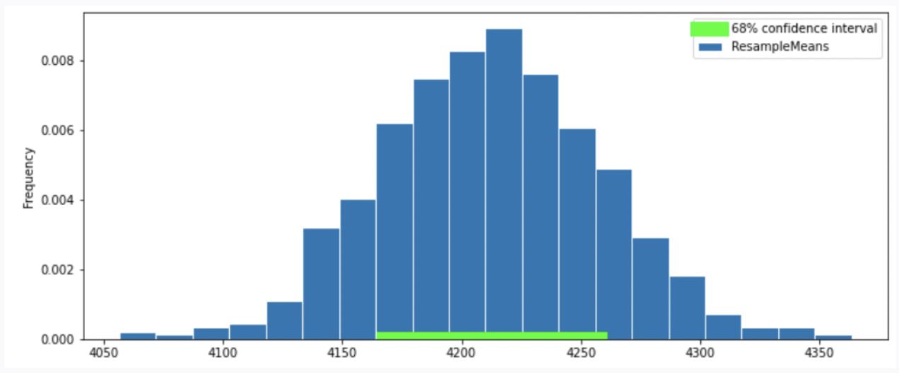
To better estimate the population mean, we bootstrapped our sample and plotted a histogram of the resample means, then took the middle 68 percent of those values to get a confidence interval. Which option below shows the histogram of the resample means and the confidence interval we found?
Option 1
Option 2
Option 3
Option 4
Answer: Option 2
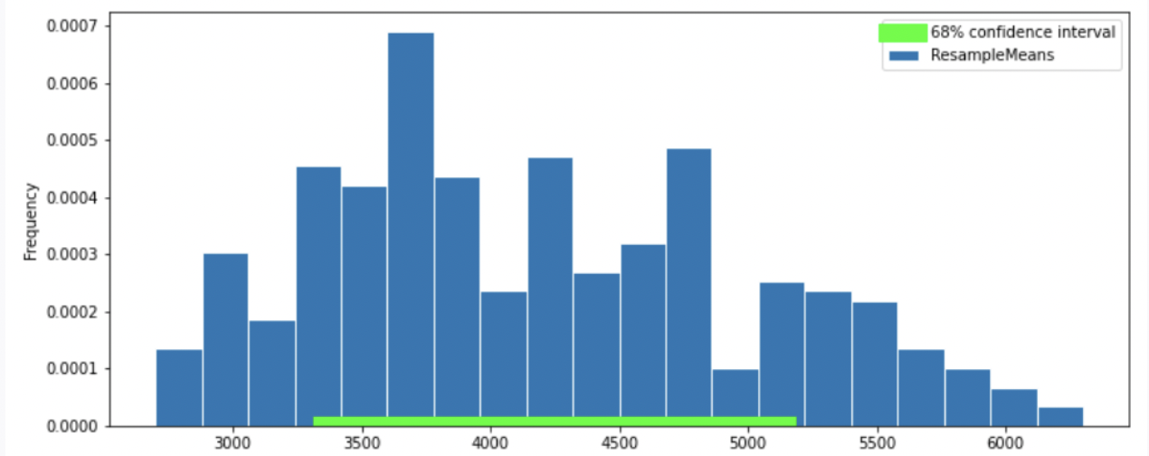
Recall, according to the Central Limit Theorem (CLT), the probability distribution of the sum or mean of a large random sample drawn with replacement will be roughly normal, regardless of the distribution of the population from which the sample is drawn.
Thus, our graph should have a normal distribution. We eliminate Option 4.
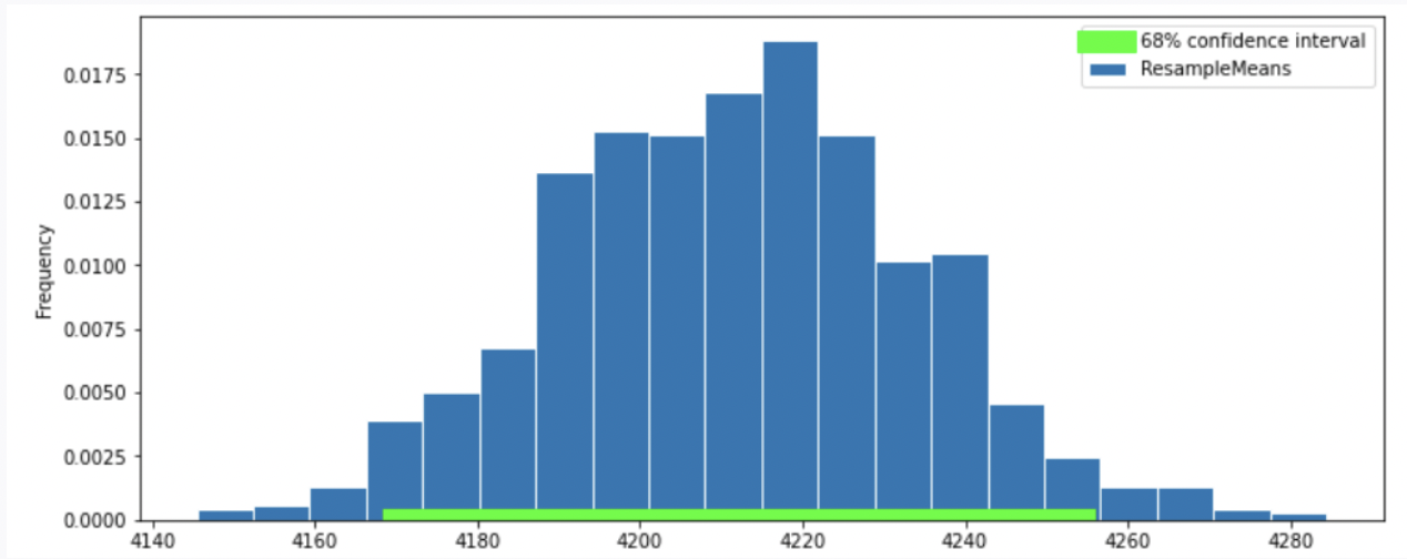
Recall that the standard normal curve has inflection points at z = +-1, which is 68% proportion of a normal distribution.(inflection point is where a curve goes from “opening down” to “opening up”) Since we have a confidence intervel of 68% in this question, by looking at the inflection point, we can eliminate Option 3
To compute the SD of the sample mean’s distribution, when we don’t know the population’s SD, we can use the sample’s SD (840): \text{SD of Distribution of Possible Sample Means} \approx \frac{\text{Sample SD}}{\sqrt{\text{sample size}}} = \frac{840}{\sqrt{330}} \approx 46.24
Recall: proportion with z SDs of the mean
| Percent in Range | All Distributions (via Chebyshev’s Inequality) | Normal Distributions |
|---|---|---|
| \text{average} \pm 1 \ \text{SD} | \geq 0\% | \approx 68\% |
| \text{average} \pm 2\text{SDs} | \geq 75\% | \approx 95\% |
| \text{average} \pm 3\text{SDs} | \geq 88\% | \approx 99.73\% |
In this question, we want 68% confidence interval, given that the distribution of sample mean is roughly normal, our CI should have range \text{sample mean} \pm 1 \ \text{SD}. Thus, the interval is approximately [4200-46.24 = 4153.76, 4200+46.24=4246.24]. We compare the 68% CI in Option 1, 2 and we choose Option 2 since it has a 68% CI with approximately the same interval.
The average score on this problem was 66%.
Suppose boot_means is an array of the resampled means.
Fill in the blanks below so that [left, right] is a 68%
confidence interval for the true mean mass of penguins.
left = np.percentile(boot_means, __(a)__)
right = np.percentile(boot_means, __(b)__)
[left, right]
What goes in blank (a)? What goes in blank (b)?
Answer: (a) 16 (b) 84
Recall, np.percentile(array, p) computes the
pth percentile of the numbers in array. To
compute the 68% CI, we need to know the percentile of left tail and
right tail.
left percentile = (1-0.68)/2 = (0.32)/2 = 0.16 so we have 16th percentile
right percentile = 1-((1-0.68)/2) = 1-((0.32)/2) = 1-0.16 = 0.84 so we have 84th percentile
The average score on this problem was 94%.
Which of the following is a correct interpretation of this confidence interval? Select all that apply.
There is an approximately 68% chance that mean weight of all penguins in Antarctica falls within the bounds of this confidence interval.
Approximately 68% of penguin weights in our sample fall within the bounds of this confidence interval.
Approximately 68% of penguin weights in the population fall within the bounds of this interval.
If we created many confidence intervals using the same method, approximately 68% of them would contain the mean weight of all penguins in Antarctica.
None of the above
Answer: Option 4 (If we created many confidence intervals using the same method, approximately 68% of them would contain the mean weight of all penguins in Antarctica.)
Recall, what a k% confidence level states is that approximately k% of the time, the intervals you create through this process will contain the true population parameter.
In this question, our population parameter is the mean weight of all penguins in Antarctica. So 86% of the time, the intervals you create through this process will contain the mean weight of all penguins in Antarctica. This is the same as Option 4. However, it will be false if we state it in the reverse order (Option 1) since our population parameter is already fixed.
The average score on this problem was 81%.
Now let’s study the relationship between a penguin’s bill length (in millimeters) and mass (in grams). Suppose we’re given that
Which of the four scatter plots below describe the relationship between bill length and body mass, based on the information provided in the question?
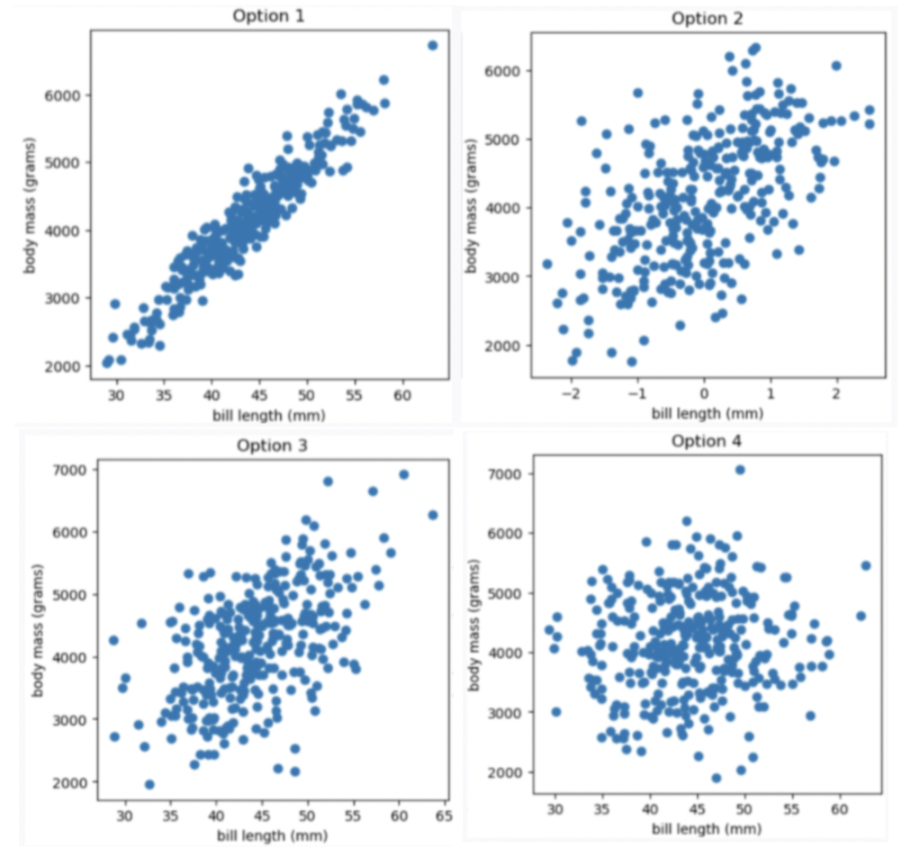
Option 1
Option 2
Option 3
Option 4
Answer Option 3
Given the correlation coefficient is 0.55, bill length and body mass has a moderate positive correlation. We eliminate Option 1 (strong correlation) and Option 4 (weak correlation).
Given the average bill length is 44 mm, we expect our x-axis to have 44 at the middle, so we eliminate Option 2
The average score on this problem was 91%.
Suppose we want to find the regression line that uses bill length, x, to predict body mass, y. The line is of the form y = mx +\ b. What are m and b?
What is m? Give your answer as a number without any units, rounded to three decimal places.
What is b? Give your answer as a number without units, rounded to three decimal places.
Answer: m = 77, b = 812
m = r \cdot \frac{\text{SD of }y }{\text{SD of }x} = 0.55 \cdot \frac{840}{6} = 77 b = \text{mean of }y - m \cdot \text{mean of }x = 4200-77 \cdot 44 = 812
The average score on this problem was 92%.
What is the predicted body mass (in grams) of a penguin whose bill length is 44 mm? Give your answer as a number without any units, rounded to three decimal places.
Answer: 4200
y = mx\ +\ b = 77 \cdot 44 + 812 = 3388 +812 = 4200
The average score on this problem was 95%.
A particular penguin had a predicted body mass of 6800 grams. What is that penguin’s bill length (in mm)? Give your answer as a number without any units, rounded to three decimal places.
Answer: 77.766
In this question, we want to compute x value given y value y = mx\ +\ b y - b = mx \frac{y - b}{m} = x\ \ \text{(m is nonzero)} x = \frac{y - b}{m} = \frac{6800 - 812}{77} = \frac{5988}{77} \approx 77.766
The average score on this problem was 88%.
Below is the residual plot for our regression line.
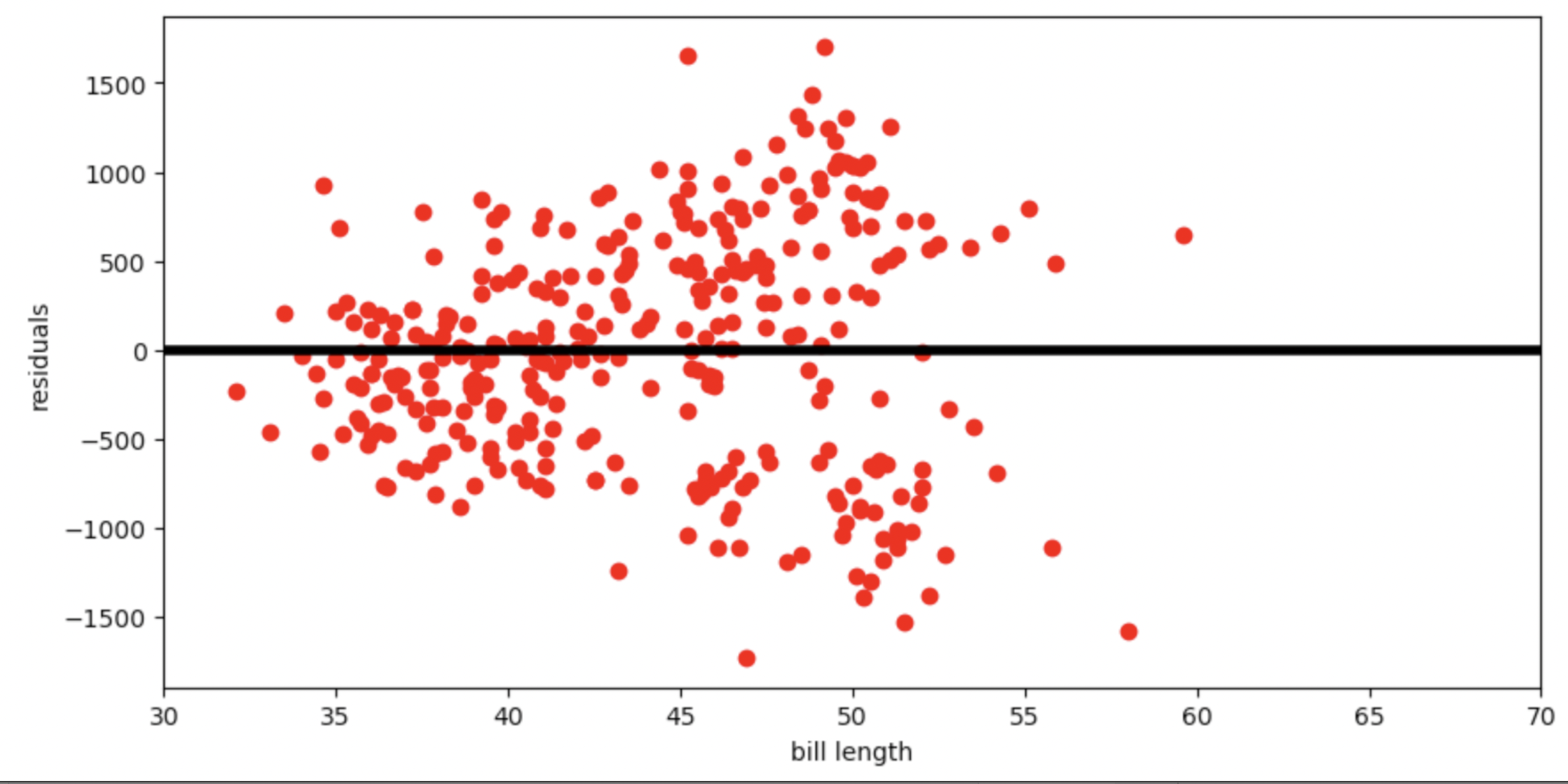
Which of the following is a valid conclusion that we can draw solely from the residual plot above?
For this dataset, there is another line with a lower root mean squared error
The root mean squared error of the regression line is 0
The accuracy of the regression line’s predictions depends on bill length
The relationship between bill length and body mass is likely non-linear
None of the above
Answer: The accuracy of the regression line’s predictions depends on bill length
The vertical spread in this residual plot is uneven, which implies that the regression line’s predictions aren’t equally accurate for all inputs. This doesn’t necessarily mean that fitting a nonlinear curve would be better. It just impacts how we interpret the regression line’s predictions.
The average score on this problem was 40%.
Each individual penguin in our dataset is of a certain species (Adelie, Chinstrap, or Gentoo) and comes from a particular island in Antarctica (Biscoe, Dream, or Torgerson). There are 330 penguins in our dataset, grouped by species and island as shown below.
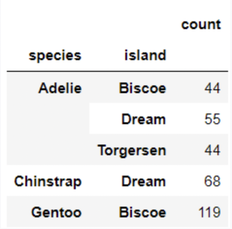
Suppose we pick one of these 330 penguins, uniformly at random, and name it Chester.
What is the probability that Chester comes from Dream island? Give your answer as a number between 0 and 1, rounded to three decimal places.
Answer: 0.373
P(Chester comes from Dream island) = # of penguins in dream island / # of all penguins in the data = \frac{55+68}{330} \approx 0.373
The average score on this problem was 94%.
If we know that Chester comes from Dream island, what is the probability that Chester is an Adelie penguin? Give your answer as a number between 0 and 1, rounded to three decimal places.
Answer: 0.447
P(Chester is an Adelie penguin given that Chester comes from Dream island) = # of Adelie penguins from Dream island / # of penguins from Dream island = \frac{55}{55+68} \approx 0.447
The average score on this problem was 91%.
If we know that Chester is not from Dream island, what is the probability that Chester is not an Adelie penguin? Give your answer as a number between 0 and 1, rounded to three decimal places.
Answer: 0.575
Method 1
P(Chester is not an Adelie penguin given that Chester is not from Dream island) = # of penguins that are not Adelie penguins from islands other than Dream island / # of penguins in island other than Dream island = \frac{119\ \text{(eliminate all penguins that are Adelie or from Dream island, only Gentoo penguins from Biscoe are left)}}{44+44+119} \approx 0.575
Method 2
P(Chester is not an Adelie penguin given that Chester is not from Dream island) = 1- (# of penguins that are Adelie penguins from islands other than Dream island / # of penguins in island other than Dream island) = 1-\frac{44+44}{44+44+119} \approx 0.575
The average score on this problem was 85%.
We’re now interested in investigating the differences between the masses of Adelie penguins and Chinstrap penguins. Specifically, our null hypothesis is that their masses are drawn from the same population distribution, and any observed differences are due to chance only.
Below, we have a snippet of working code for this hypothesis test,
for a specific test statistic. Assume that adelie_chinstrap
is a DataFrame of only Adelie and Chinstrap penguins, with just two
columns – 'species' and 'mass'.
stats = np.array([])
num_reps = 500
for i in np.arange(num_reps):
    # --- line (a) starts ---
    shuffled = np.random.permutation(adelie_chinstrap.get('species'))
    # --- line (a) ends ---

    # --- line (b) starts ---
    with_shuffled = adelie_chinstrap.assign(species=shuffled)
    # --- line (b) ends ---

    grouped = with_shuffled.groupby('species').mean()

    # --- line (c) starts ---
    stat = grouped.get('mass').iloc[0] - grouped.get('mass').iloc[1]
    # --- line (c) ends ---

stats = np.append(stats, stat)Which of the following statements best describe the procedure above?
This is a standard hypothesis test, and our test statistic is the total variation distance between the distribution of Adelie masses and Chinstrap masses
This is a standard hypothesis test, and our test statistic is the difference between the expected proportion of Adelie penguins and the proportion of Adelie penguins in our resample
This is a permutation test, and our test statistic is the total variation distance between the distribution of Adelie masses and Chinstrap masses
This is a permutation test, and our test statistic is the difference in the mean Adelie mass and mean Chinstrap mass
Answer: This is a permutation test, and our test statistic is the difference in the mean Adelie mass and mean Chinstrap mass (Option 4)
Recall, a permutation test helps us decide whether two random samples
come from the same distribution. This test matches our goal of testing
whether the masses of Adelie penguins and Chinstrap penguins are drawn
from the same population distribution. The code above are also doing
steps of a permutation test. In part (a), it shuffles
'species' and stores the shuffled series to
shuffled. In part (b), it assign the shuffled series of
values to 'species' column. Then, it uses
grouped = with_shuffled.groupby('species').mean() to
calculate the mean of each species. In part (c), it computes the
difference between mean mass of the two species by first getting the
'mass' column and then accessing mean mass of each group
(Adelie and Chinstrap) with positional index 0 and
1.
The average score on this problem was 98%.
Currently, line (c) (marked with a comment) uses .iloc. Which of the following options compute the exact same statistic as line (c) currently does?
Option 1:
stat = grouped.get('mass').loc['Adelie'] - grouped.get('mass').loc['Chinstrap']Option 2:
stat = grouped.get('mass').loc['Chinstrap'] - grouped.get('mass').loc['Adelie']Option 1 only
Option 2 only
Both options
Neither option
Answer: Option 1 only
We use df.get(column_name).iloc[positional_index] to
access the value in a column with positional_index.
Similarly, we use df.get(column_name).loc[index] to access
value in a column with its index. Remember
grouped is a DataFrame that
groupby('species'), so we have species name
'Adelie' and 'Chinstrap' as index for
grouped.
Option 2 is incorrect since it does subtraction in the reverse order
which results in a different stat compared to
line(c). Its output will be -1
\cdot stat. Recall, in
grouped = with_shuffled.groupby('species').mean(), we use
groupby() and since 'species' is a column with
string values, our index will be sorted in alphabetical order. So,
.iloc[0] is 'Adelie' and .iloc[1]
is 'Chinstrap'.
The average score on this problem was 81%.
Is it possible to re-write line (c) in a way that uses
.iloc[0] twice, without any other uses of .loc
or .iloc?
Yes, it’s possible
No, it’s not possible
Answer: Yes, it’s possible
There are multiple ways to achieve this. For instance
stat = grouped.get('mass').iloc[0] - grouped.sort_index(ascending = False).get('mass').iloc[0].
The average score on this problem was 64%.
What would happen if we removed line (a), and replaced
line (b) with
with_shuffled = adelie_chinstrap.sample(adelie_chinstrap.shape[0], replace=False)Select the best answer.
This would still run a valid hypothesis test
This would not run a valid hypothesis test, as all values in the
stats array would be exactly the same
This would not run a valid hypothesis test, even though there would
be several different values in the stats array
This would not run a valid hypothesis test, as it would incorporate information about Gentoo penguins
Answer: This would not run a valid hypothesis test,
as all values in the stats array would be exactly the same
(Option 2)
Recall, DataFrame.sample(n, replace = False) (or
DataFrame.sample(n) since replace = False is
by default) returns a DataFrame by randomly sampling n rows
from the DataFrame, without replacement. Since our n is
adelie_chinstrap.shape[0], and we are sampling without
replacement, we will get the exactly same Dataframe (though the order of
rows may be different but the stats array would be exactly
the same).
The average score on this problem was 87%.
What would happen if we removed line (a), and replaced
line (b) with
with_shuffled = adelie_chinstrap.sample(adelie_chinstrap.shape[0], replace=True)Select the best answer.
This would still run a valid hypothesis test
This would not run a valid hypothesis test, as all values in the
stats array would be exactly the same
This would not run a valid hypothesis test, even though there would
be several different values in the stats array
This would not run a valid hypothesis test, as it would incorporate information about Gentoo penguins
Answer: This would not run a valid hypothesis test,
even though there would be several different values in the
stats array (Option 3)
Recall, DataFrame.sample(n, replace = True) returns a
new DataFrame by randomly sampling n rows from the
DataFrame, with replacement. Since we are sampling with replacement, we
will have a DataFrame which produces a stats array with
some different values. However, recall, the key idea behind a
permutation test is to shuffle the group labels. So, the above code does
not meet this key requirement since we only want to shuffle the
"species" column without changing the size of the two
species. However, the code may change the size of the two species.
The average score on this problem was 66%.
What would happen if we replaced line (a) with
with_shuffled = adelie_chinstrap.assign(
    species=np.random.permutation(adelie_chinstrap.get('species'))
)
and replaced line (b) with
with_shuffled = with_shuffled.assign(
    mass=np.random.permutation(adelie_chinstrap.get('mass'))
)
Select the best answer.
This would still run a valid hypothesis test
This would not run a valid hypothesis test, as all values in the
stats array would be exactly the same
This would not run a valid hypothesis test, even though there would
be several different values in the stats array
This would not run a valid hypothesis test, as it would incorporate information about Gentoo penguins
Answer: This would still run a valid hypothesis test (Option 1)
Our goal for the permutation test is to randomly assign masses to
groups, without changing group sizes. The above code shuffles
'species' and 'mass' columns and assigns them
back to the DataFrame. This fulfills our goal.
The average score on this problem was 81%.
Suppose we run the code for the hypothesis test and see the following empirical distribution for the test statistic. In red is the observed statistic.
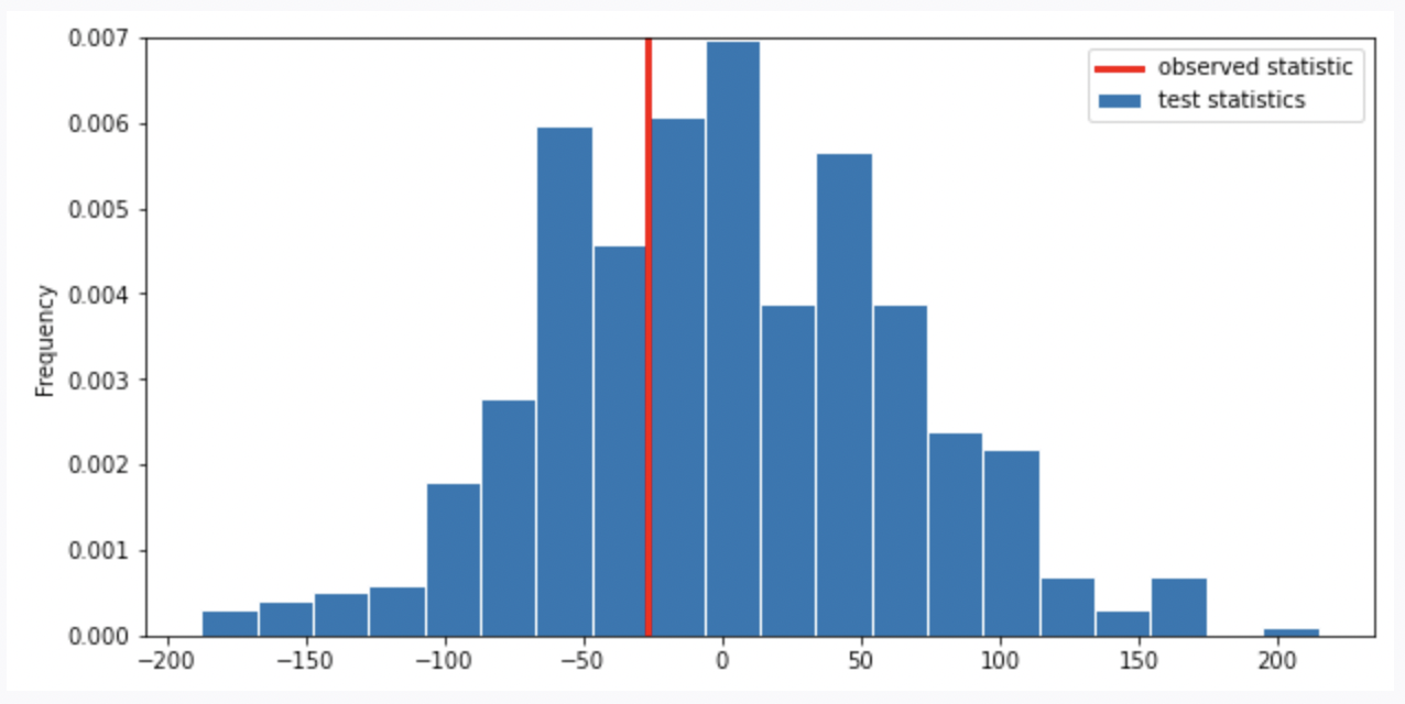
Suppose our alternative hypothesis is that Chinstrap penguins weigh more on average than Adelie penguins. Which of the following is closest to the p-value for our hypothesis test?
0
\frac{1}{4}
\frac{1}{3}
\frac{2}{3}
\frac{3}{4}
1
Answer: \frac{1}{3}
Recall, the p-value is the chance, under the null hypothesis, that the test statistic is equal to the value that was observed in the data or is even further in the direction of the alternative. Thus, we compute the proportion of the test statistic that is equal or less than the observed statistic. (It is less than because less than corresponds to the alternative hypothesis “Chinstrap penguins weigh more on average than Adelie penguins”. Recall, when computing the statistic, we use Adelie’s mean mass minus Chinstrap’s mean mass. If Chinstrap’s mean mass is larger, the statistic will be negative, the direction of less than the observed statistic).
Thus, we look at the proportion of area less than or on the red line (which represents observed statistic), it is around \frac{1}{3}.
The average score on this problem was 80%.
At the San Diego Model Railroad Museum, there are different admission prices for children, adults, and seniors. Over a period of time, as tickets are sold, employees keep track of how many of each type of ticket are sold. These ticket counts (in the order child, adult, senior) are stored as follows.
admissions_data = np.array([550, 1550, 400])Complete the code below so that it creates an array
admissions_proportions with the proportions of tickets sold
to each group (in the order child, adult, senior).
def as_proportion(data):
    return __(a)__

admissions_proportions = as_proportion(admissions_data)
What goes in blank (a)?
Answer: data/data.sum()
To calculate proportion for each group, we divide each value in the array (tickets sold to each group) by the sum of all values (total tickets sold). Remember values in an array can be processed as a whole.
The average score on this problem was 95%.
The museum employees have a model in mind for the proportions in which they sell tickets to children, adults, and seniors. This model is stored as follows.
model = np.array([0.25, 0.6, 0.15])We want to conduct a hypothesis test to determine whether the admissions data we have is consistent with this model. Which of the following is the null hypothesis for this test?
Child, adult, and senior tickets might plausibly be purchased in proportions 0.25, 0.6, and 0.15.
Child, adult, and senior tickets are purchased in proportions 0.25, 0.6, and 0.15.
Child, adult, and senior tickets might plausibly be purchased in proportions other than 0.25, 0.6, and 0.15.
Child, adult, and senior tickets, are purchased in proportions other than 0.25, 0.6, and 0.15.
Answer: Child, adult, and senior tickets are purchased in proportions 0.25, 0.6, and 0.15. (Option 2)
Recall, null hypothesis is the hypothesis that there is no significant difference between specified populations, any observed difference being due to sampling or experimental error. So, we assume the distribution is the same as the model.
The average score on this problem was 88%.
Which of the following test statistics could we use to test our hypotheses? Select all that could work.
sum of differences in proportions
sum of squared differences in proportions
mean of differences in proportions
mean of squared differences in proportions
none of the above
Answer: sum of squared differences in proportions, mean of squared differences in proportions (Option 2, 4)
We need to use squared difference to avoid the case that large positive and negative difference cancel out in the process of calculating sum or mean, resulting in small sum of difference or mean of difference that does not reflect the actual deviation. So, we eliminate Option 1 and 3.
The average score on this problem was 77%.
Below, we’ll perform the hypothesis test with a different test statistic, the mean of the absolute differences in proportions.
Recall that the ticket counts we observed for children, adults, and
seniors are stored in the array
admissions_data = np.array([550, 1550, 400]), and that our
model is model = np.array([0.25, 0.6, 0.15]).
For our hypothesis test to determine whether the admissions data is
consistent with our model, what is the observed value of the test
statistic? Give your answer as a number between 0 and 1, rounded to
three decimal places. (Suppose that the value you calculated is assigned
to the variable observed_stat, which you will use in later
questions.)
Answer: 0.02
We first calculate the proportion for each value in
admissions_data \frac{550}{550+1550+400} = 0.22 \frac{1550}{550+1550+400} = 0.62 \frac{400}{550+1550+400} = 0.16 So, we have
the distribution of the admissions_data
Then, we calculate the observed value of the test statistic (the mean of the absolute differences in proportions) \frac{|0.22-0.25|+|0.62-0.6|+|0.16-0.15|}{number\ of\ goups} =\frac{0.03+0.02+0.01}{3} = 0.02
The average score on this problem was 82%.
Now, we want to simulate the test statistic 10,000 times under the
assumptions of the null hypothesis. Fill in the blanks below to complete
this simulation and calculate the p-value for our hypothesis test.
Assume that the variables admissions_data,
admissions_proportions, model, and
observed_stat are already defined as specified earlier in
the question.
simulated_stats = np.array([])
for i in np.arange(10000):
    simulated_proportions = as_proportions(np.random.multinomial(__(a)__, __(b)__))
    simulated_stat = __(c)__
    simulated_stats = np.append(simulated_stats, simulated_stat)

p_value = __(d)__
What goes in blank (a)? What goes in blank (b)? What goes in blank (c)? What goes in blank (d)?
Answer: (a) admissions_data.sum() (b)
model (c)
np.abs(simulated_proportions - model).mean() (d)
np.count_nonzero(simulated_stats >= observed_stat) / 10000
Recall, in np.random.multinomial(n, [p_1, ..., p_k]),
n is the number of experiments, and
[p_1, ..., p_k] is a sequence of probability. The method
returns an array of length k in which each element contains the number
of occurrences of an event, where the probability of the ith event is
p_i.
We want our simulated_proportion to have the same data
size as admissions_data, so we use
admissions_data.sum() in (a).
Since our null hypothesis is based on model, we simulate
based on distribution in model, so we have
model in (b).
In (c), we compute the mean of the absolute differences in
proportions. np.abs(simulated_proportions - model) gives us
a series of absolute differences, and .mean() computes the
mean of the absolute differences.
In (d), we calculate the p_value. Recall, the
p_value is the chance, under the null hypothesis, that the
test statistic is equal to the value that was observed in the data or is
even further in the direction of the alternative.
np.count_nonzero(simulated_stats >= observed_stat) gives
us the number of simulated_stats greater than or equal to
the observed_stat in the 10000 times simulations, so we
need to divide it by 10000 to compute the proportion of
simulated_stats greater than or equal to the
observed_stat, and this gives us the
p_value.
The average score on this problem was 79%.
True or False: the p-value represents the probability that the null hypothesis is true.
True
False
Answer: False
Recall, the p-value is the chance, under the null hypothesis, that the test statistic is equal to the value that was observed in the data or is even further in the direction of the alternative. It only gives us the strength of evidence in favor of the null hypothesis, which is different from “the probability that the null hypothesis is true”.
The average score on this problem was 64%.
The new statistic that we used for this hypothesis test, the mean of
the absolute differences in proportions, is in fact closely related to
the total variation distance. Given two arrays of length three,
array_1 and array_2, suppose we compute the
mean of the absolute differences in proportions between
array_1 and array_2 and store the result as
madp. What value would we have to multiply
madp by to obtain the total variation distance
array_1 and array_2? Give your answer as a
number rounded to three decimal places.
Answer: 1.5
Recall, the total variation distance (TVD) is the sum of the absolute differences in proportions, divided by 2. When we compute the mean of the absolute differences in proportions, we are computing the sum of the absolute differences in proportions, divided by the number of groups (which is 3). Thus, to get TVD, we first multiply our current statistics (the mean of the absolute differences in proportions) by 3, we get the sum of the absolute differences in proportions. Then according to the definition of TVD, we divide this value by 2. Thus, we have \text{current statistics}\cdot 3 / 2 = \text{current statistics}\cdot 1.5.
The average score on this problem was 65%.