← return to practice.dsc10.com
Instructor(s): Suraj Rampure, Puoya Tabaghi, Janine Tiefenbruck
This exam was administered in-person. The exam was closed-notes, except students were provided a copy of the DSC 10 Reference Sheet. No calculators were allowed. Students had 3 hours to take this exam.
Note (groupby / pandas 2.0): Pandas 2.0+ no longer
silently drops columns that can’t be aggregated after a
groupby, so code written for older pandas may behave
differently or raise errors. In these practice materials we use
.get() to select the column(s) we want after
.groupby(...).mean() (or other aggregations) so that our
solutions run on current pandas. On real exams you will not be penalized
for omitting .get() when the old behavior would have
produced the same answer.
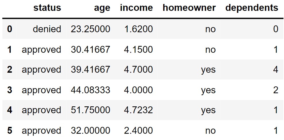
Credit cards allow consumers to make purchases by borrowing money and paying it back later. Credit card companies are wary of granting this borrowing ability to consumers who may not be able to pay back their debt. Therefore, potential credit card carriers must submit an application that contains information about themselves and their history of paying back debt.
The DataFrame apps contains application data for a
random sample of 1,000 applicants for a particular credit card from the
1990s. The columns are:
"status" (str): Whether the credit card application
was approved: "approved" or "denied" values
only.
"age" (float): The applicant’s age, in years, to the
nearest twelfth of a year.
"income" (float): The applicant’s annual income, in
tens of thousands of dollars.
"homeowner" (str): Whether the credit card applicant
owns their own home: "yes" or "no" values
only.
"dependents" (int): The number of dependents, or
individuals that rely on the applicant as a primary source of income,
such as children.
The first few rows of apps are shown below, though
remember that apps has 1,000 rows.
Throughout this exam, we will refer to apps
repeatedly.
Assume that:
Each applicant only submitted a single application.
We have already run import babypandas as bpd and
import numpy as np.
Tip: Open this page in another tab, so that it is easy to refer to this data description as you work through the exam.
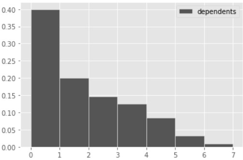
In this question, we’ll explore the number of dependents of each applicant. To begin, let’s define the variable dep_counts as follows.
dep_counts = apps.groupby("dependents").count().get(["status"])
The visualization below shows the distribution of the numbers of dependents per applicant. Note that every applicant has 6 or fewer dependents.
Use dep_counts and the visualization above to answer the
following questions.
What is the type of the variable dep_counts?
array
Series
DataFrame
Answer: DataFrame
As usual, .groupby produces a new DataFrame. Then we use
.get on this DataFrame with a list as the input, which
produces a DataFrame with just one column. Remember that
.get("status") produces a Series, but
.get(["status"]) produces a DataFrame
The average score on this problem was 78%.
What type of data visualization is shown above?
line plot
scatter plot
bar chart
histogram
Answer: histogram
This is a histogram because the number of dependents per applicant is a numerical variable. It makes sense, for example, to subtract the number of dependents for two applicants to see how many more dependents one applicant has than the other. Histograms show distributions of numerical variables.
The average score on this problem was 91%.
How many of the 1,000 applicants in apps have 2 or more
dependents? Give your answer as an integer.
Answer: 400
The bars of a density histogram have a combined total area of 1, and the area in any bar represents the proportion of values that fall in that bin.
In tihs problem, we want the total area of the bins corresponding to 2 or more dependents. Since this involves 5 bins, whose exact heights are unclear, we will instead calculate the proportion of all applicants with 0 or 1 dependents, and then subtract this proportion from 1.
Since the width of each bin is 1, we have for each bin, \begin{align*} \text{Area} &= \text{Height} \cdot \text{Width}\\ \text{Area} &= \text{Height}. \end{align*}
Since the height of the first bar is 0.4, this means a proportion of 0.4 applicants have 0 dependents. Similarly, since the height of the second bar is 0.2, a proportion of 0.2 applicants have 1 dependent. This means 1-(0.4+0.2) = 0.4 proportion of applicants have 2 or more dependents. Since there are 1,000 applicants total, this is 400 applicants.
The average score on this problem was 82%.
Define the DataFrame dependents_status as follows.
dependents_status = apps.groupby(["dependents", "status"]).count()
What is the maximum number of rows that
dependents_status could have? Give your answer as an
integer.
Answer: 14
When we group by multiple columns, the resulting DataFrame has one
row for each combination of values in those columns. Since there are 7
possible values for "dependents" (0, 1, 2, 3, 4, 5, 6) and
2 possible values for "status" ("approved",
"denied"), this means there are 7\cdot 2 = 14 possible combinations of values
for these two columns.
The average score on this problem was 59%.
Recall that dep_counts is defined as follows.
dep_counts = apps.groupby("dependents").count().get(["status"])
Below, we define several more variables.
variable1 = dep_counts[dep_counts.get("status") >= 2].sum()

variable2 = dep_counts[dep_counts.index > 2].get("status").sum()

variable3 = (dep_counts.get("status").sum()
            - dep_counts[dep_counts.index < 2].get("status").sum())

variable4 = dep_counts.take(np.arange(2, 7)).get("status").sum()

variable5 = (dep_counts.get("status").sum()
            - dep_counts.get("status").loc[1]
            - dep_counts.get("status").loc[2])
Which of these variables are equal to your answer from part (c)? Select all that apply.
variable1
variable2
variable3
variable4
variable5
None of the above.
Answer: variable3,
variable4
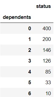
First, the DataFrame dep_counts is indexed by
"dependents" and has just one column, called
"status" containing the number of applicants with each
number of dependents. For example, dep_counts may look like
the DataFrame shown below.
variable1 does not work because it doesn’t make sense to
query with the condition dep_counts.get("status") >= 2.
In the example dep_counts shown above, all rows would
satisfy this condition, but not all rows correspond to applicants with 2
or more dependents. We should be querying based on the values in the
index instead.
variable2 is close but it uses a strict inequality
> where it should use >= because we want
to include applicants with 2 dependents.
variable3 is correct. It uses the same approach we used
in part (c). That is, in order to calculate the number of applicants
with 2 or more dependents, we calculate the total number of applicants
minus the number of applicants with less than 2 dependents.
variable4 works as well. The strategy here is to keep
only the rows that correspond to 2 or more dependents. Recall that
np.arange(2, 7) evaluates to the array
np.array([2, 3, 4, 5, 6]). Since we are told that each
applicant has 6 or fewer dependents, keeping only these rows
correspondings to keeping all applicants with 2 or more dependents.
variable5 does not work because it subtracts away the
applicants with 1 or 2 dependents, leaving the applicants with 0, 3, 4,
5, or 6 dependents. This is not what we want.
The average score on this problem was 77%.
Next, we define variables x and y as
follows.
x = dep_counts.index.values
y = dep_counts.get("status")Note: If idx is the index of a Series or
DataFrame, idx.values gives the values in idx
as an array.
Which of the following expressions evaluate to the mean number of dependents? Select all that apply.
np.mean(x * y)
x.sum() / y.sum()
(x * y / y.sum()).sum()
np.mean(x)
(x * y).sum() / y.sum()
None of the above.
Answer: (x * y / y.sum()).sum(),
(x * y).sum() / y.sum()
We know that x is
np.array([0, 1, 2, 3, 4, 5, 6]) and y is a
Series containing the number of applicants with each number of
dependents. We don’t know the exact values of the data in
y, but we do know there are 7 elements that sum to 1000,
the first two of which are 400 and 200.
np.mean(x * y) does not work because x * y
has 7 elements, so np.mean(x * y) is equivalent to
sum(x * y) / 7, but the mean number of dependents should be
sum(x * y) / 1000 since there are 1000 applicants.
x.sum() / y.sum() evaluates to \frac{21}{1000} regardless of how many
applicants have each number of dependents, so it must be incorrect.
(x * y / y.sum()).sum() works. We can think of
y / y.sum() as a Series containing the proportion of
applicants with each number of dependents. For example, the first two
entries of y / y.sum() are 0.4 and 0.2. When we multiply
this Series by x and sum up all 7 entries, the result is a
weighted average of the different number of dependents, where the
weights are given by the proportion of applicants with each number of
dependents.
np.mean(x) evaluates to 3 regardless of how many
applicants have each number of dependents, so it must be incorrect.
(x * y).sum() / y.sum() works because the numerator
(x * y).sum() represents the total number of dependents
across all 1,000 applicants and the denominator is the number of
applicants, or 1,000. The total divided by the count gives the mean
number of dependents.
The average score on this problem was 71%.
What does the expression y.iloc[0] / y.sum() evaluate
to? Give your answer as a fully simplified
fraction.
Answer: 0.4
y.iloc[0] represents the number of applicants with 0
dependents, which is 400. y.sum() represents the total
number of applicants, which is 1,000. So the ratio of these is 0.4.
The average score on this problem was 73%.
For each application in apps, we want to assign an age
category based on the value in the "age" column, according
to the table below.
"age" |
age category |
|---|---|
| under 25 | "young adult" |
| at least 25, but less than 50 | "middle aged" |
| at least 50, but less than 75 | "older adult" |
| 75 or over | "elderly" |
cat_names = ["young adult", "middle aged", "older adult", "elderly"]

def age_to_bin(one_age):
    '''Returns the age category corresponding to one_age.'''
    one_age = __(a)__
    bin_pos = __(b)__
    return cat_names[bin_pos]

binned_ages = __(c)__
apps_cat = apps.assign(age_category = binned_ages)Which of the following is a correct way to fill in blanks (a) and (b)?
| Blank (a) | Blank (b) | |
|---|---|---|
| Option 1 | 75 - one_age |
round(one_age / 25) |
| Option 2 | min(75, one_age) |
one_age / 25 |
| Option 3 | 75 - one_age |
int(one_age / 25) |
| Option 4 | min(75, one_age) |
int(one_age / 25) |
| Option 5 | min(74, one_age) |
round(one_age / 25) |
Option 1
Option 2
Option 3
Option 4
Option 5
Answer: Option 4
The line one_age = min(75, one_age) either leaves
one_age alone or sets it equal to 75 if the age was higher
than 75, which means anyone over age 75 is considered to be 75 years old
for the purposes of classifying them into age categories. From the
return statement, we know we need our value for bin_pos to
be either 0, 1 ,2 or 3 since cat_names has a length of 4.
When we divide one_age by 25, we get a decimal number that
represents how many times 25 fits into one_age. We want to
round this number down to get the number of whole copies of 25
that fit into one_age. If that value is 0, it means the
person is a "young adult", if that value is 1, it means
they are "middle aged", and so on. The rounding down
behavior that we want is accomplished by
int(one_age/25).
The average score on this problem was 76%.
Which of the following is a correct way to fill in blank (c)?
age to bin(apps.get("age"))
apps.get("age").apply(age to bin)
apps.get("age").age to bin()
apps.get("age").apply(age to bin(one age))
Answer:
apps.get("age").apply(age to bin)
We want our result to be a Series because the next line in the code
assigns it to a DataFrame. We also need to use the .apply()
method to apply our function to the entirety of the "age"
column. The .apply() method only takes in the name of a
function and not its variables, as it treats the entries of the column
as the variables directly.
The average score on this problem was 96%.
Which of the following is a correct alternate implementation of the age to bin function? Select all that apply.
Option 1:
def age_to_bin(one_age):
    bin_pos = 3
    if one_age < 25:
        bin_pos = 0
    if one_age < 50:
        bin_pos = 1
    if one_age < 75:
        bin_pos = 2
    return cat_names[bin_pos]
Option 2:
def age_to_bin(one_age):
    bin_pos = 3
    if one_age < 75:
        bin_pos = 2
    if one_age < 50:
        bin_pos = 1
    if one_age < 25:
        bin_pos = 0
    return cat_names[bin_pos]
Option 3:
def age_to_bin(one_age):
    bin_pos = 0
    for cutoff in np.arange(25, 100, 25):
        if one_age >= cutoff:
            bin_pos = bin_pos + 1
    return cat_names[bin_pos]
Option 4:
def age_to_bin(one_age):
    bin_pos = -1
    for cutoff in np.arange(0, 100, 25):
        if one_age >= cutoff:
            bin_pos = bin_pos + 1
        return cat_names[bin_pos]
Option 1
Option 2
Option 3
Option 4
None of the above.
Answer: Option 2 and Option 3
Option 1 doesn’t work for inputs less than 25. For example, on an
input of 10, every condition is satsified, so bin_pos will
be set to 0, then 1, then 2, meaning the function will return
"older adult" instead of "young adult".
Option 2 reverses the order of the conditions, which ensures that
even when a number satisfies many conditions, the last one it satisfies
determines the correct bin_pos. For example, 27 would
satisfy the first 2 conditions but not the last one, and the function
would return "middle aged" as expected.
In option 3, np.arange(25, 100, 25) produces
np.array([25,50,75]). The if condition checks
the whether the age is at least 25, then 50, then 75. For every time
that it is, it adds to bin_pos, otherwise it keeps
bin_pos. At the end, bin_pos represents the
number of these values that the age is greater than or equal to, which
correctly determines the age category.
Option 4 is equivalent to option 3 except for two things. First,
bin_pos starts at -1, but since 0 is included in the set of
cutoff values, the first time through the loop will set
bin_pos to 0, as in Option 3. This change doesn’t affect
the behavior of the funtion. The other change, however, is that the
return statement is inside the for-loop, which
does change the behavior of the function dramatically. Now the
for-loop will only run once, checking whether the age is at
least 0 and then returning immediately. Since ages are always at least
0, this function will return "young adult" on every input,
which is clearly incorrect.
The average score on this problem was 62%.
We want to determine the number of "middle aged"
applicants whose applications were denied. Fill in the blank below so
that count evaluates to that number.
df = apps_cat.________.reset_index()
count = df[(df.get("age_category") == "middle aged") &
           (df.get("status") == "denied")].get("income").iloc[0]
What goes in the blank?
Answer:
groupby(["age_category", "status"]).count()
We can tell by the line in which count is defined that
df needs to have columns called
"age category", "status", and
"income" with one row such that the values in these columns
are "middle aged", "denied", and the number of
such applicants, respectively. Since there is one row corresponding to a
possible combination of values for "age category" and
"status", this suggests we need to group by the pair of
columns, since .groupby produces a DataFrame with one row
for each possible combination of values in the columns we are grouping
by. Since we want to know how many individuals have this combination of
values for "age category" and "status", we
should use .count() as the aggregation method. Another clue
to to use .groupby is the presence of
.reset_index() which is needed to query based on columns
called "age category" and "status".
The average score on this problem was 78%.
The total variation distance between the distributions of
"age category" for approved applications and denied
applications is 0.4.
One of the visualizations below shows the distributions of
"age category" for approved applications and denied
applications. Which visualization is it?
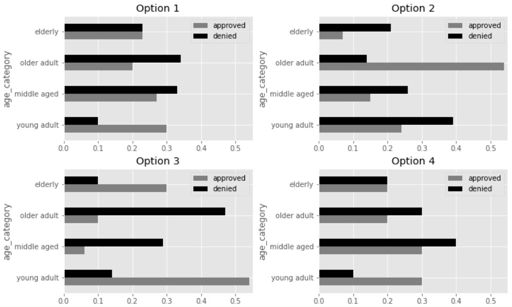
Answer: Option 2
TVD represents the total overrepresentation of one distrubtion, summed across all categories. To find the TVD visually, we can estimate how much each bar for approved applications extends beyond the corresponding bar for denied applications in each bar chart.
In Option 1, the approved bar extends beyond the denied bar only in
the "young adult" category, and by 0.2, so the TVD for
Option 1 is 0.2. In Option 2, the approved bar extends beyond the denied
bar only in the "older adult" category, and by 0.4, so the
TVD for Option 2 is 0.4. In Option 3, the approved bar extends beyond
the denied bar in "elderly" by 0.2 and in
"young adult" by 0.4, for a TVD of 0.6. In Option 4, the
approved bar extends beyond the denied bar in
"young adult only" by 0.2, for a TVD of 0.2.
Note that even without knowing the exact lengths of the bars in Option 2, we can still conclude that Option 2 is correct by process of elimination, since it’s the only one whose TVD appears close to 0.4
The average score on this problem was 60%.
In apps, our sample of 1,000 credit card applications,
500 of the applications come from homeowners and 500 come from people
who don’t own their own home. In this sample, homeowner ages have a mean
of 40 and standard deviation of 10. We want to use the bootstrap method
to compute a confidence interval for the mean age of a homeowner in the
population of all credit card applicants.
Note: This problem is out of scope; it covers material no longer included in the course.
Suppose our computer is too slow to bootstrap 10,000 times, and instead can only bootstrap 20 times. Here are the 20 resample means, sorted in ascending order: \begin{align*} &37, 38, 39, 39, 40, 40, 40, 40, 41 , 41, \\ &42, 42, 42, 42, 42, 42, 43, 43, 43 , 44 \end{align*} What are the left and right endpoints of a bootstrapped 80% confidence interval for the population mean? Use the mathematical definition of percentile.
Answer: Left endpoint = 38, Right endpoint = 43
To find an 80% confidence interval, we need to find the 10th and 90th percentiles of the resample means. Using the mathematical definiton of percentile, the 10th percentile is at position 0.1*20 = 2 when we count starting with 1. Since 38 is the second element of the sorted data, that is the left endpoint of our confidence interval.
The average score on this problem was 63%.
Similarly, the 90th percentile is at position 0.9*20 = 18 when we count starting with 1. Since 43 is the 18th element of the sorted data, that is the right endpoint of our confidence interval.
The average score on this problem was 65%.
Note: This problem is out of scope; it covers material no longer included in the course.
True or False: Using the mathematical definition of percentile, the 50th percentile of the bootstrapped distribution above equals its median.
True
False
Answer: False
The 50th percentile according to the mathematial definition is the element at position 0.5*20 10 when we count starting with 1. The 10th element is 41. However, the median of a data set with 20 elements is halfway between the 10th and 11th values. So the median in this case is 41.5.
The average score on this problem was 79%.
Consider the following three quantities:
pop_mean, the unknown mean age of homeowners in the
population of all credit card applicants.
sample_mean, the mean age of homeowners in our
sample of 500 applications in apps. We know this is
40.
resample_mean, the mean age of homeowners in one
particular resample of the applications in apps.
Which of the following statements about the relationship between these three quantities are guaranteed to be true? Select all that apply.
If sample_mean is less than pop_mean, then
resample_mean is also less than pop_mean.
The mean of sample_mean and resample_mean
is closer to pop_mean than either of the two values
individually.
resample_mean is closer than sample_mean to
pop_mean.
resample_mean is further than sample_mean
from pop_mean.
None of the above.
Answer: None of the above.
Whenever we take a sample from a population, there is no guaranteed
relationship between the mean of the sample and the mean of the
population. Sometimes the mean of the sample comes out larger than the
population mean, sometimes smaller. We know this from the CLT which says
that the distribution of the sample mean is centered at the
population mean. Similarly, when we resample from an original mean, the
resample mean could be larger or smaller than the original sample’s
mean. The three quantities pop_mean,
sample_mean, and resample_mean can be in any
relative order. This means none of the statements listed here are
necessarily true.
The average score on this problem was 37%.
In apps, our sample of 1,000 credit card applications,
applicants who were approved for the credit card have fewer dependents,
on average, than applicants who were denied. The mean number of
dependents for approved applicants is 0.98, versus 1.07 for denied
applicants.
To test whether this difference is purely due to random chance, or whether the distributions of the number of dependents for approved and denied applicants are truly different in the population of all credit card applications, we decide to perform a permutation test.
Consider the incomplete code block below.
def shuffle_status(df):
    shuffled_status = np.random.permutation(df.get("status"))
    return df.assign(status=shuffled_status).get(["status", "dependents"])

def test_stat(df):
    grouped = df.groupby("status").mean().get("dependents")
    approved = grouped.loc["approved"]
    denied = grouped.loc["denied"]
    return __(a)__

stats = np.array([])
for i in np.arange(10000):
    shuffled_apps = shuffle_status(apps)
    stat = test_stat(shuffled_apps)
    stats = np.append(stats, stat)

p_value = np.count_nonzero(__(b)__) / 10000
Below are six options for filling in blanks (a) and (b) in the code above.
| Blank (a) | Blank (b) | |
|---|---|---|
| Option 1 | denied - approved |
stats >= test_stat(apps) |
| Option 2 | denied - approved |
stats <= test_stat(apps) |
| Option 3 | approved - denied |
stats >= test_stat(apps) |
| Option 4 | np.abs(denied - approved) |
stats >= test_stat(apps) |
| Option 5 | np.abs(denied - approved) |
stats <= test_stat(apps) |
| Option 6 | np.abs(approved - denied) |
stats >= test_stat(apps) |
The correct way to fill in the blanks depends on how we choose our null and alternative hypotheses.
Suppose we choose the following pair of hypotheses.
Null Hypothesis: In the population, the number of dependents of approved and denied applicants come from the same distribution.
Alternative Hypothesis: In the population, the number of dependents of approved applicants and denied applicants do not come from the same distribution.
Which of the six presented options could correctly fill in blanks (a) and (b) for this pair of hypotheses? Select all that apply.
Option 1
Option 2
Option 3
Option 4
Option 5
Option 6
None of the above.
Answer: Option 4, Option 6
For blank (a), we want to choose a test statistic that helps us
distinguish between the null and alternative hypotheses. The alternative
hypothesis says that denied and approved
should be different, but it doesn’t say which should be larger. Options
1 through 3 therefore won’t work, because high values and low values of
these statistics both point to the alternative hypothesis, and moderate
values point to the null hypothesis. Options 4 through 6 all work
because large values point to the alternative hypothesis, and small
values close to 0 suggest that the null hypothesis should be true.
For blank (b), we want to calculate the p-value in such a way that it
represents the proportion of trials for which the simulated test
statistic was equal to the observed statistic or further in the
direction of the alternative. For all of Options 4 through 6, large
values of the test statistic indicate the alternative, so we need to
calculate the p-value with a >= sign, as in Options 4
and 6.
While Option 3 filled in blank (a) correctly, it did not fill in blank (b) correctly. Options 4 and 6 fill in both blanks correctly.
The average score on this problem was 78%.
Now, suppose we choose the following pair of hypotheses.
Null Hypothesis: In the population, the number of dependents of approved and denied applicants come from the same distribution.
Alternative Hypothesis: In the population, the number of dependents of approved applicants is smaller on average than the number of dependents of denied applicants.
Which of the six presented options could correctly fill in blanks (a) and (b) for this pair of hypotheses? Select all that apply.
Answer: Option 1
As in the previous part, we need to fill blank (a) with a test
statistic such that large values point towards one of the hypotheses and
small values point towards the other. Here, the alterntive hypothesis
suggests that approved should be less than
denied, so we can’t use Options 4 through 6 because these
can only detect whether approved and denied
are not different, not which is larger. Any of Options 1 through 3
should work, however. For Options 1 and 2, large values point towards
the alternative, and for Option 3, small values point towards the
alternative. This means we need to calculate the p-value in blank (b)
with a >= symbol for the test statistic from Options 1
and 2, and a <= symbol for the test statistic from
Option 3. Only Options 1 fills in blank (b) correctly based on the test
statistic used in blank (a).
The average score on this problem was 83%.
Option 6 from the start of this question is repeated below.
| Blank (a) | Blank (b) | |
|---|---|---|
| Option 6 | np.abs(approved - denied) |
stats >= test_stat(apps) |
We want to create a new option, Option 7, that replicates the behavior of Option 6, but with blank (a) filled in as shown:
| Blank (a) | Blank (b) | |
|---|---|---|
| Option 7 | approved - denied |
Which expression below could go in blank (b) so that Option 7 is equivalent to Option 6?
np.abs(stats) >= test_stat(apps)
stats >= np.abs(test_stat(apps))
np.abs(stats) >= np.abs(test_stat(apps))
np.abs(stats >= test_stat(apps))
Answer:
np.abs(stats) >= np.abs(test_stat(apps))
First, we need to understand how Option 6 works. Option 6 produces
large values of the test statistic when approved is very
different from denied, then calculates the p-value as the
proportion of trials for which the simulated test statistic was larger
than the observed statistic. In other words, Option 6 calculates the
proportion of trials in which approved and
denied are more different in a pair of random samples than
they are in the original samples.
For Option 7, the test statistic for a pair of random samples may
come out very large or very small when approved is very
different from denied. Similarly, the observed statistic
may come out very large or very small when approved and
denied are very different in the original samples. We want
to find the proportion of trials in which approved and
denied are more different in a pair of random samples than
they are in the original samples, which means we want the proportion of
trials in which the absolute value of approved - denied in
a pair of random samples is larger than the absolute value of
approved - denied in the original samples.
The average score on this problem was 56%.
In our implementation of this permutation test, we followed the
procedure outlined in lecture to draw new pairs of samples under the
null hypothesis and compute test statistics — that is, we randomly
assigned each row to a group (approved or denied) by shuffling one of
the columns in apps, then computed the test statistic on
this random pair of samples.
Let’s now explore an alternative solution to drawing pairs of samples under the null hypothesis and computing test statistics. Here’s the approach:
"dependents"
column as the new “denied” sample, and the values at the at the bottom
of the resulting "dependents" column as the new “approved”
sample. Note that we don’t necessarily split the DataFrame exactly in
half — the sizes of these new samples depend on the number of “denied”
and “approved” values in the original DataFrame!Once we generate our pair of random samples in this way, we’ll compute the test statistic on the random pair, as usual. Here, we’ll use as our test statistic the difference between the mean number of dependents for denied and approved applicants, in the order denied minus approved.
Fill in the blanks to complete the simulation below.
Hint: np.random.permutation shouldn’t appear
anywhere in your code.
    def shuffle_all(df):
        '''Returns a DataFrame with the same rows as df, but reordered.'''
        return __(a)__

    def fast_stat(df):
        # This function does not and should not contain any randomness.
        denied = np.count_nonzero(df.get("status") == "denied")
        mean_denied = __(b)__.get("dependents").mean()
        mean_approved = __(c)__.get("dependents").mean()
        return mean_denied - mean_approved

    stats = np.array([])
    for i in np.arange(10000):
        stat = fast_stat(shuffle_all(apps))
stats = np.append(stats, stat)Answer: The blanks should be filled in as follows:
df.sample(df.shape[0])df.take(np.arange(denied))df.take(np.arange(denied, df.shape[0]))For blank (a), we are told to return a DataFrame with the same rows
but in a different order. We can use the .sample method for
this question. We want each row of the input DataFrame df
to appear once, so we should sample without replacement, and we should
have has many rows in the output as in df, so our sample
should be of size df.shape[0]. Since sampling without
replacement is the default behavior of .sample, it is
optional to specify replace=False.
The average score on this problem was 59%.
For blank (b), we need to implement the strategy outlined, where
after we shuffle the DataFrame, we use the values at the top of the
DataFrame as our new “denied sample. In a permutation test, the two
random groups we create should have the same sizes as the two original
groups we are given. In this case, the size of the”denied” group in our
original data is stored in the variable denied. So we need
the rows in positions 0, 1, 2, …, denied - 1, which we can
get using df.take(np.arange(denied)).
The average score on this problem was 39%.
For blank (c), we need to get all remaining applicants, who form the
new “approved” sample. We can .take the rows corresponding
to the ones we didn’t put into the “denied” group. That is, the first
applicant who will be put into this group is at position
denied, and we’ll take all applicants from there onwards.
We should therefore fill in blank (c) with
df.take(np.arange(denied, df.shape[0])).
For example, if apps had only 10 rows, 7 of them
corresponding to denied applications, we would shuffle the rows of
apps, then take rows 0, 1, 2, 3, 4, 5, 6 as our new
“denied” sample and rows 7, 8, 9 as our new “approved” sample.
The average score on this problem was 38%.
Choose the best tool to answer each of the following questions. Note the following:
Are incomes of applicants with 2 or fewer dependents drawn randomly from the distribution of incomes of all applicants?
Hypothesis Testing
Permutation Testing
Bootstrapping
Anwser: Hypothesis Testing
This is a question of whether a certain set of incomes (corresponding to applicants with 2 or fewer dependents) are drawn randomly from a certain population (incomes of all applicants). We need to use hypothesis testing to determine whether this model for how samples are drawn from a population seems plausible.
The average score on this problem was 47%.
What is the median income of credit card applicants with 2 or fewer dependents?
Hypothesis Testing
Permutation Testing
Bootstrapping
Anwser: Bootstrapping
The question is looking for an estimate a specific parameter (the median income of applicants with 2 or fewer dependents), so we know boostrapping is the best tool.
The average score on this problem was 88%.
Are credit card applications approved through a random process in which 50% of applications are approved?
Hypothesis Testing
Permutation Testing
Bootstrapping
Anwser: Hypothesis Testing
The question asks about the validity of a model in which applications are approved randomly such that each application has a 50% chance of being approved. To determine whether this model is plausible, we should use a standard hypothesis test to simulate this random process many times and see if the data generated according to this model is consistent with our observed data.
The average score on this problem was 74%.
Is the median income of applicants with 2 or fewer dependents less than the median income of applicants with 3 or more dependents?
Hypothesis Testing
Permutation Testing
Bootstrapping
Anwser: Permutation Testing
Recall, a permutation test helps us decide whether two random samples come from the same distribution. This question is about whether two random samples for different groups of applicants have the same distribution of incomes or whether they don’t because one group’s median incomes is less than the other.
The average score on this problem was 57%.
What is the difference in median income of applicants with 2 or fewer dependents and applicants with 3 or more dependents?
Hypothesis Testing
Permutation Testing
Bootstrapping
Anwser: Bootstrapping
The question at hand is looking for a specific parameter value (the difference in median incomes for two different subsets of the applicants). Since this is a question of estimating an unknown parameter, bootstrapping is the best tool.
The average score on this problem was 63%.
In this question, we’ll explore the relationship between the ages and incomes of credit card applicants.
The credit card company that owns the data in apps,
BruinCard, has decided not to give us access to the entire
apps DataFrame, but instead just a sample of
apps called small_apps. We’ll start by using
the information in small_apps to compute the regression
line that predicts the age of an applicant given their income.
For an applicant with an income that is \frac{8}{3} standard deviations above the
mean income, we predict their age to be \frac{4}{5} standard deviations above the
mean age. What is the correlation coefficient, r, between incomes and ages in
small_apps? Give your answer as a fully simplified
fraction.
Answer: r = \frac{3}{10}
To find the correlation coefficient r we use the equation of the regression line in standard units and solve for r as follows. \begin{align*} \text{predicted } y_{\text{(su)}} &= r \cdot x_{\text{(su)}} \\ \frac{4}{5} &= r \cdot \frac{8}{3} \\ r &= \frac{4}{5} \cdot \frac{3}{8} \\ r &= \frac{3}{10} \end{align*}
The average score on this problem was 52%.
Now, we want to predict the income of an applicant given their age.
We will again use the information in small_apps to find the
regression line. The regression line predicts that an applicant whose
age is \frac{4}{5} standard deviations
above the mean age has an income that is s standard deviations above the mean income.
What is the value of s? Give your
answer as a fully simplified fraction.
Answer: s = \frac{6}{25}
We again use the equation of the regression line in standard units, with the value of r we found in the previous part. \begin{align*} \text{predicted } y_{\text{(su)}} &= r \cdot x_{\text{(su)}} \\ s &= \frac{3}{10} \cdot \frac{4}{5} \\ s &= \frac{6}{25} \end{align*}
Notice that when we predict income based on age, our predictions are different than when we predict age based on income. That is, the answer to this question is not \frac{8}{3}. We can think of this phenomenon as a consequence of regression to the mean which means that the predicted variable is always closer to average than the original variable. In part (a), we start with an income of \frac{8}{3} standard units and predict an age of \frac{4}{5} standard units, which is closer to average than \frac{8}{3} standard units. Then in part (b), we start with an age of \frac{4}{5} and predict an income of \frac{6}{25} standard units, which is closer to average than \frac{4}{5} standard units. This happens because whenever we make a prediction, we multiply by r which is less than one in magnitude.
The average score on this problem was 21%.
BruinCard has now taken away our access to both apps and
small_apps, and has instead given us access to an even
smaller sample of apps called mini_apps. In
mini_apps, we know the following information:
We use the data in mini_apps to find the regression line
that will allow us to predict the income of an applicant given their
age. Just to test the limits of this regression line, we use it to
predict the income of an applicant who is -2 years old,
even though it doesn’t make sense for a person to have a negative
age.
Let I be the regression line’s prediction of this applicant’s income. Which of the following inequalities are guaranteed to be satisfied? Select all that apply.
I < 0
I < \text{mean income}
| I - \text{mean income}| \leq | \text{mean age} + 2 |
\dfrac{| I - \text{mean income}|}{\text{standard deviation of incomes}} \leq \dfrac{| \text{mean age} + 2 |}{\text{standard deviation of ages}}
None of the above.
Answer: I < \text{mean income}, \dfrac{| I - \text{mean income}|}{\text{standard deviation of incomes}} \leq \dfrac{| \text{mean age} + 2 |}{\text{standard deviation of ages}}
To understand this answer, we will investigate each option.
This option asks whether income is guaranteed to be negative. This is not necessarily true. For example, it’s possible that the slope of the regression line is 2 and the intercept is 10, in which case the income associated with a -2 year old would be 6, which is positive.
This option asks whether the predicted income is guaranteed to be lower than the mean income. It helps to think in standard units. In standard units, the regression line goes through the point (0, 0) and has slope r, which we are told is positive. This means that for a below-average x, the predicted y is also below average. So this statement must be true.
First, notice that | \text{mean age} + 2 | = | -2 - \text{mean age}|, which represents the horizontal distance betweeen these two points on the regression line: (\text{mean age}, \text{mean income}), (-2, I). Likewise, | I - \text{mean income}| represents the vertical distance between those same two points. So the inequality can be interpreted as a question of whether the rise of the regression line is less than or equal to the run, or whether the slope is at most 1. That’s not guaranteed when we’re working in original units, as we are here, so this option is not necessarily true.
Since standard deviation cannot be negative, we have \dfrac{| I - \text{mean income}|}{\text{standard deviation of incomes}} = \left| \dfrac{I - \text{mean income}}{\text{standard deviation of incomes}} \right| = I_{\text{(su)}}. Similarly, \dfrac{|\text{mean age} + 2|}{\text{standard deviation of ages}} = \left| \dfrac{-2 - \text{mean age}}{\text{standard deviation of ages}} \right| = -2_{\text{(su)}}. So this option is asking about whether the predicted income, in standard units, is guaranteed to be less (in absolute value) than the age. Since we make predictions in standard units using the equation of the regression line \text{predicted } y_{\text{(su)}} = r \cdot x_{\text{(su)}} and we know |r|\leq 1, this means |\text{predicted } y_{\text{(su)}}| \leq | x_{\text{(su)}}|. Applying this to ages (x) and incomes (y), this says exactly what the given inequality says. This is the phenomenon we call regression to the mean.
The average score on this problem was 69%.
Yet again, BruinCard, the company that gave us access to
apps, small_apps, and mini_apps,
has revoked our access to those three DataFrames and instead has given
us micro_apps, an even smaller sample of
apps.
Using micro_apps, we are again interested in finding the
regression line that will allow us to predict the income of an applicant
given their age. We are given the following information:
Suppose the standard deviation of incomes in micro_apps
is an integer multiple of the standard deviation of ages in
micro_apps. That is,
\text{standard deviation of income} = k \cdot \text{standard deviation of age}.
What is the value of k? Give your answer as an integer.
Answer: k = 4
To find this answer, we’ll use the definition of the regression line in original units, which is \text{predicted } y = mx+b, where m = r \cdot \frac{\text{SD of } y}{\text{SD of }x}, \: \: b = \text{mean of } y - m \cdot \text{mean of } x
Next we substitute these value for m and b into \text{predicted } y = mx + b, interpret x as age and y as income, and use the given information to find k. \begin{align*} \text{predicted } y &= mx+b \\ \text{predicted } y &= r \cdot \frac{\text{SD of } y}{\text{SD of }x} \cdot x+ \text{mean of } y - r \cdot \frac{\text{SD of } y}{\text{SD of }x} \cdot \text{mean of } x\\ \text{predicted income}&= r \cdot \frac{\text{SD of income}}{\text{SD of age}} \cdot \text{age}+ \text{mean income} - r \cdot \frac{\text{SD of income}}{\text{SD of age}} \cdot \text{mean age} \\ \frac{31}{2}&= -\frac{1}{3} \cdot k \cdot 24+ \frac{7}{2} + \frac{1}{3} \cdot k \cdot 33 \\ \frac{31}{2}&= -8k+ \frac{7}{2} + 11k \\ \frac{31}{2}&= 3k+ \frac{7}{2} \\ 3k &= \frac{31}{2} - \frac{7}{2} \\ 3k &= 12 \\ k &= 4 \end{align*}
Another way to solve this problem uses the equation of the regression line in standard units and the definition of standard units.
\begin{align*} \text{predicted } y_{\text{(su)}} &= r \cdot x_{\text{(su)}} \\ \frac{\text{predicted income} - \text{mean income}}{\text{SD of income}} &= r \cdot \frac{\text{age} - \text{mean age}}{\text{SD of age}} \\ \frac{\frac{31}{2} - \frac{7}{2}}{k\cdot \text{SD of age}} &= -\frac{1}{3} \cdot \frac{24 - 33}{\text{SD of age}} \\ \frac{12}{k\cdot \text{SD of age}} &= -\frac{1}{3} \cdot \frac{-9}{\text{SD of age}} \\ \frac{12}{k\cdot \text{SD of age}} &= \frac{3}{\text{SD of age}} \\ \frac{k\cdot \text{SD of age}}{\text{SD of age}} &= \frac{12}{3}\\ k &= 4 \end{align*}
The average score on this problem was 45%.
Below, we define a new DataFrame called
seven_apps and display it fully.
seven_apps = apps.sample(7).sort_values(by="dependents", ascending=False)
seven_apps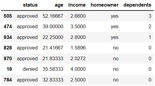
Consider the process of resampling 7 rows from
seven_apps with replacement, and computing the
maximum number of dependents in the resample.
If we take one resample, what is the probability that the maximum number of dependents in the resample is less than 3? Leave your answer unsimplified.
Answer: \left( 1 - \frac{1}{7}\right)^7 = \left( \frac{6}{7}\right)^7
Of the 7 rows in the seven_apps DataFrame, there are 6
rows that have a value less than 3 in the dependents
column. This means that if we were to sample one row
from seven_apps, there would be a \frac{6}{7} chance of selecting one of the
rows that has less than 3 dependents. The question is asking what the
probability that the maximum number of dependents in the resample is
less than 3. One resample of the DataFrame is equivalent to sampling one
row from seven_apps 7 different times, without replacement.
So the probability of getting a row with less than 3 dependents, 7 times
consecutively, is \left(
\frac{6}{7}\right)^7.
The average score on this problem was 47%.
If we take 50 resamples, what is the probability that the maximum number of dependents is never 3, in any resample? Leave your answer unsimplified.
Answer: \left[ \left( 1 - \frac{1}{7}\right)^7 \right]^{50} = \left( \frac{6}{7}\right)^{350}
We know from the previous part of this question that the probability
of one resample of seven_apps having a maximum number of
dependents less than 3 is \left(
\frac{6}{7}\right)^7. Now we must repeat this process 50 times
independently, and so the probability that all 50 resamples have a
maximum number of dependents less than 3 is \left(\left( \frac{6}{7}\right)^{7}\right)^{50} =
\left( \frac{6}{7}\right)^{350}. Another way to interpret this is
that we must select 350 rows, one a time, such that none of them are the
one row containing 3 dependents.
The average score on this problem was 41%.
If we take 50 resamples, what is the probability that the maximum number of dependents is 3 in every resample? Leave your answer unsimplified.
Answer: \left[1 - \left( 1 - \frac{1}{7}\right)^7 \right]^{50} = \left[1 - \left( \frac{6}{7}\right)^7 \right]^{50}
We’ll first take a look at the probability of one
resample of seven_apps having the maximum number
of dependents be 3. In order for this to happen, at least one row of the
7 selected for the resample must be the row containing 3 dependents. The
probability of getting this row at least once is equal to the complement
of the probability of never getting this row, which we calculated in
part (a) to be \left(
\frac{6}{7}\right)^7. Therefore, the probability that at least
one row in the resample has 3 dependents, is 1
-\left( \frac{6}{7}\right)^7.
Now that we know the probability of getting one resample where the maximum number of dependents is 3, we can calculate the probability that the same thing happens in 50 independent resamples by multiplying this probability by itself 50 times. Therefore, the probability that the maximum number of dependents is 3 in each of 50 resamples is \left[1 - \left( \frac{6}{7}\right)^7 \right]^{50}.
The average score on this problem was 27%.
At TritonCard, a new UCSD alumni-run credit card company, applications are approved at random. Each time someone submits an application, a TritonCard employee rolls a fair six-sided die two times. If both rolls are the same even number — that is, if both are 2, both are 4, or both are 6 — TritonCard approves the application. Otherwise, they reject it.
You submit k identical TritonCard applications. The probability that at least one of your applications is approved is of the form 1-\left(\frac{a}{b}\right)^k. What are the values of a and b? Give your answers as integers such that the fraction \frac{a}{b} is fully simplified.
Answer: a = 11, b = 12
The format of the answer suggests we should use the complement rule. The opposite of at least one application being approved is that no applications are approved, or equivalently, all applications are denied.
Consider one application. Its probability of being approved is \frac{3}{6}*\frac{1}{6} = \frac{3}{36} = \frac{1}{12} because we need to get any one of the three even numbers on the first roll, then the second roll must match the first. So one application has a probability of being denied equal to \frac{11}{12}.
Therefore, the probability that all k applications are denied is \left(\frac{11}{12}\right)^k. The probability that this does not happen, or at least one is approved, is given by 1-\left(\frac{11}{12}\right)^k.
The average score on this problem was 41%.
Every TritonCard credit card has a 3-digit security code on the back, where each digit is a number 0 through 9. There are 1,000 possible 3-digit security codes: 000, 001, \dots, 998, 999.
Tony, the CEO of TritonCard, wants to only issue credit cards whose security codes satisfy all of the following criteria:
The first digit is odd.
The middle digit is 0.
The last digit is even.
Tony doesn’t have a great way to generate security codes meeting these three criteria, but he does know how to generate security codes with three unique (distinct) digits. That is, no number appears in the security code more than once. So, Tony decides to randomly select a security code from among those with three unique digits. If the randomly selected security code happens to meet the desired criteria, TritonCard will issue a credit card with this security code, otherwise Tony will try his process again.
What is the probability that Tony’s first randomly selected security code satisfies the given criteria? Give your answer as a fully simplified fraction.
Answer: \frac{1}{36}
Imagine generating a security code with three unique digits by selecting one digit at a time. In other words, we would need to select three values without replacement from the set of digits 0, 1, 2, \dots, 9. The probability that the first digit is odd is \frac{5}{10}. Then, assuming the first digit is odd, the probability of the middle digit being 0 is \frac{1}{9} since only nine digits are remaining, and one of them must be 0. Then, assuming we have chosen an odd number for the first digit and 0 or the middle digit, there are 8 remaining digits we could select, and only 4 of them are even, so the probability of the third digit being even is \frac{4}{8}. Multiplying these all together gives the probability that all three criteria are satisfied: \frac{5}{10} \cdot \frac{1}{9} \cdot \frac{4}{8} = \frac{1}{36}
The average score on this problem was 38%.
Daphne, the newest employee at TritonCard, wants to try a different way of generating security codes. She decides to randomly select a 3-digit code from among all 1,000 possible security codes (i.e. the digits are not necessarily unique). As before, if the code randomly selected code happens to meet the desired criteria, TritonCard will issue a credit card with this security code, otherwise Daphne will try her process again.
What is the probability that Daphne’s first randomly selected security code satisfies the given criteria? Give your answer as a fully simplified fraction.
Answer: \frac{1}{40}
We’ll use a similar strategy as in the previous part. This time, however, we need to select three values with replacement from the set of digits 0, 1, 2, \dots, 9. The probability that the first digit is odd is \frac{5}{10}. Then, assuming the first digit is odd, the probability of the middle digit being 0 is \frac{1}{10} since any of the ten digits can be chosen, and one of them is 0. Then, assuming we have chosen an odd number for the first digit and 0 or the middle digit, the probability of getting an even number for the third digit is \frac{5}{10}, which actually does not depend at all on what we selected for the other digits. In fact, when we sample with replacement, the probabilities of each digit satisfying the given criteria don’t depend on whether the other digits satisfied the given criteria (in other words, they are independent). This is different from the previous part, where knowledge of previous digits satisfying the criteria informed the chances of the next digit satisfying the criteria. So for this problem, we can really just think of each of the three digits separately and multiply their probabilties of meeting the desired criteria: \frac{5}{10} \cdot \frac{1}{10} \cdot \frac{5}{10} = \frac{1}{40}
The average score on this problem was 51%.
After you graduate, you are hired by TritonCard! On your new work
computer, you install numpy, but something goes wrong with
the installation — your copy of numpy doesn’t come with
np.random.multinomial. To demonstrate your resourcefulness
to your new employer, you decide to implement your own version of
np.random.multinomial.
Below, complete the implementation of the function
manual_multinomial so that
manual_multinomial(n, p) works the same way as
np.random.multinomial(n, p). That is,
manual_multinomial should take in an integer n
and an array of probabilities p. It should return an array
containing the counts in each category when we randomly draw
n items from a categorical distribution where the
probabilities of drawing an item from each category are given in the
array p. The array returned by
manual_multinomial(n, p) should have a length of
len(p) and a sum of n.
For instance, to simulate flipping a coin five times, we could call
manual_multinomial(5, np.array([0.5, 0.5])), and the output
might look like array([2, 3]).
def manual_multinomial(n, p):
    values = np.arange(len(p))
    choices = np.random.choice(values, size=__(a)__, replace=__(b)__, p=p)
    value_counts = np.array([])
    for value in values:
        value_count = __(c)__
        value_counts = np.append(value_counts, value_count)
return value_countsWhat goes in blank (a)?
Answer: n
The size argument in np.random.choice provides the
number of samples we draw. In the manual_multinomial
function, we randomly draw n items, and so the size should
be n.
The average score on this problem was 81%.
What goes in blank (b)?
Answer: True
Here, we are using np.random.choice to simulate picking
n elements from values. We draw with
replacement since we are allowed to have repeated elements. For example,
if we were flipping a coin five times, we would need to have repeated
elements, since there are only two possible outcomes of a coin flip but
we are flipping the coin more than two times.
The average score on this problem was 79%.
What goes in blank (c)?
Answer:
np.count_nonzero(choices == value)
The choices variable contains an array of the
n randomly drawn values selected from values.
In each iteration of the for-loop, we want to count the number of
elements in choices that are equal to the given
value. To do this, we can use
np.count_nonzero(choices == value). In the end,
value_counts is an array that says how many times we
selected 0, how many times we selected 1, and so on.
The average score on this problem was 37%.
The credit card company that owns the data in apps,
BruinCard, has decided not to give us access to the entire
apps DataFrame, but instead just a random sample of 100
rows of apps called hundred_apps.
We are interested in estimating the mean age of all applicants in
apps given only the data in hundred_apps. The
ages in hundred_apps have a mean of 35 and a standard
deviation of 10.
Give the endpoints of the CLT-based 95% confidence interval for the
mean age of all applicants in apps, based on the data in
hundred_apps.
Answer: Left endpoint = 33, Right endpoint = 37
According to the Central Limit Theorem, the standard deviation of the distribution of the sample mean is \frac{\text{sample SD}}{\sqrt{\text{sample size}}} = \frac{10}{\sqrt{100}} = 1. Then using the fact that the distribution of the sample mean is roughly normal, since 95% of the area of a normal curve falls within two standard deviations of the mean, we can find the endpoints of the 95% CLT-based confidence interval as 35 - 2 = 33 and 35 + 2 = 37.
We can think of this as using the formula below: \left[\text{sample mean} - 2\cdot \frac{\text{sample SD}}{\sqrt{\text{sample size}}}, \: \text{sample mean} + 2\cdot \frac{\text{sample SD}}{\sqrt{\text{sample size}}} \right]. Plugging in the appropriate quantities yields [35 - 2\cdot\frac{10}{\sqrt{100}}, 35 - 2\cdot\frac{10}{\sqrt{100}}] = [33, 37].
The average score on this problem was 67%.
BruinCard reinstates our access to apps so that we can
now easily extract information about the ages of all applicants. We
determine that, just like in hundred_apps, the ages in
apps have a mean of 35 and a standard deviation of 10. This
raises the question of how other samples of 100 rows of
apps would have turned out, so we compute 10,000 sample means as follows.
    sample_means = np.array([])
    for i in np.arange(10000):
        sample_mean = apps.sample(100, replace=True).get("age").mean()
sample_means = np.append(sample_means, sample_mean)Which of the following three visualizations best depict the
distribution of sample_means?
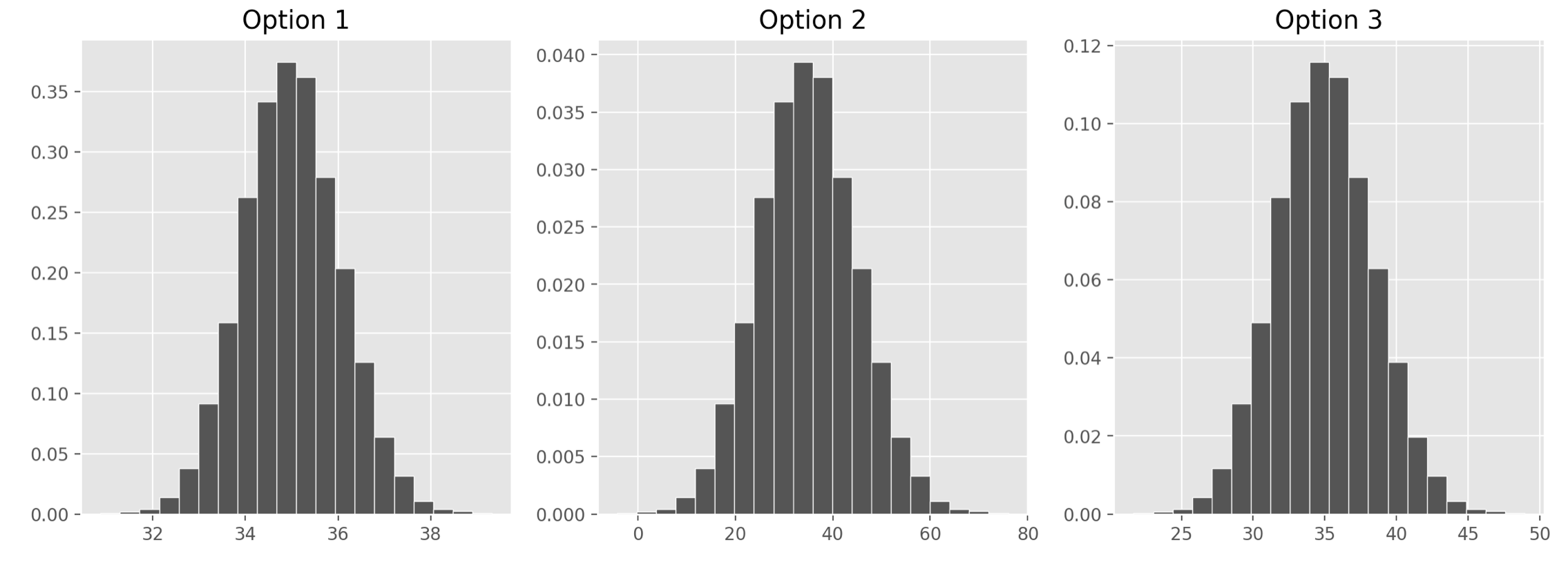
Answer: Option 1
As we found in the previous part, the distribution of the sample mean should have a standard deviation of 1. We also know it should be centered at the mean of our sample, at 35, but since all the options are centered here, that’s not too helpful. Only Option 1, however, has a standard deviation of 1. Remember, we can approximate the standard deviation of a normal curve as the distance between the mean and either of the inflection points. Only Option 1 looks like it has inflection points at 34 and 36, a distance of 1 from the mean of 35.
If you chose Option 2, you probably confused the standard deviation of our original sample, 10, with the standard deviation of the distribution of the sample mean, which comes from dividing that value by the square root of the sample size.
The average score on this problem was 57%.
Which of the following statements are guaranteed to be true? Select all that apply.
We used bootstrapping to compute sample_means.
The ages of credit card applicants are roughly normally distributed.
A CLT-based 90% confidence interval for the mean age of credit card applicants, based on the data in hundred apps, would be narrower than the interval you gave in part (a).
The expression np.percentile(sample_means, 2.5)
evaluates to the left endpoint of the interval you gave in part (a).
If we used the data in hundred_apps to create 1,000
CLT-based 95% confidence intervals for the mean age of applicants in
apps, approximately 950 of them would contain the true mean
age of applicants in apps.
None of the above.
Answer: A CLT-based 90% confidence interval for the
mean age of credit card applicants, based on the data in
hundred_apps, would be narrower than the interval you gave
in part (a).
Let’s analyze each of the options:
Option 1: We are not using bootstrapping to compute sample means
since we are sampling from the apps DataFrame, which is our
population here. If we were bootstrapping, we’d need to sample from our
first sample, which is hundred_apps.
Option 2: We can’t be sure what the distribution of the ages of
credit card applicants are. The Central Limit Theorem says that the
distribution of sample_means is roughly normally
distributed, but we know nothing about the population
distribution.
Option 3: The CLT-based 95% confidence interval that we calculated in part (a) was computed as follows: \left[\text{sample mean} - 2\cdot \frac{\text{sample SD}}{\sqrt{\text{sample size}}}, \text{sample mean} + 2\cdot \frac{\text{sample SD}}{\sqrt{\text{sample size}}} \right] A CLT-based 90% confidence interval would be computed as \left[\text{sample mean} - z\cdot \frac{\text{sample SD}}{\sqrt{\text{sample size}}}, \text{sample mean} + z\cdot \frac{\text{sample SD}}{\sqrt{\text{sample size}}} \right] for some value of z less than 2. We know that 95% of the area of a normal curve is within two standard deviations of the mean, so to only pick up 90% of the area, we’d have to go slightly less than 2 standard deviations away. This means the 90% confidence interval will be narrower than the 95% confidence interval.
Option 4: The left endpoint of the interval from part (a) was
calculated using the Central Limit Theorem, whereas using
np.percentile(sample_means, 2.5) is calculated empirically,
using the data in sample_means. Empirically calculating a
confidence interval doesn’t necessarily always give the exact same
endpoints as using the Central Limit Theorem, but it should give you
values close to those endpoints. These values are likely very similar
but they are not guaranteed to be the same. One way to see this is that
if we ran the code to generate sample_means again, we’d
probably get a different value for
np.percentile(sample_means, 2.5).
Option 5: The key observation is that if we used the data in
hundred_apps to create 1,000 CLT-based 95% confidence
intervals for the mean age of applicants in apps, all of
these intervals would be exactly the same. Given a sample, there is only
one CLT-based 95% confidence interval associated with it. In our case,
given the sample hundred_apps, the one and only CLT-based
95% confidence interval based on this sample is the one we found in part
(a). Therefore if we generated 1,000 of these intervals, either they
would all contain the parameter or none of them would. In order for a
statement like the one here to be true, we would need to collect 1,000
different samples, and calculate a confidence interval from each
one.
The average score on this problem was 49%.
Suppose variables v1, v2, v3,
and v4, have already been initialized to specific numerical
values. Right now, we don’t know what values they’ve been set to.
The function f shown below takes in a number,
v, and outputs an integer between -2 and 2, depending on
the value of v relative to v1,
v2, v3, and v4.
def f(v):
    if v <= v1:
        return -2
    elif v <= v2:
        return -1
    elif v <= v3:
        return 0
    elif v <= v4:
        return 1
    else:
        return 2
Recall that in the previous problem, we created an array called
sample_means containing 10,000 values, each of which is the
mean of a random sample of 100 applicant ages drawn from the DataFrame
apps, in which ages have a mean of 35 and a standard
deviation of 10.
When we call the function f on every value
v in sample_means, we produce a collection of
10,000 values all between -2 and 2. A density histogram of these values
is shown below.
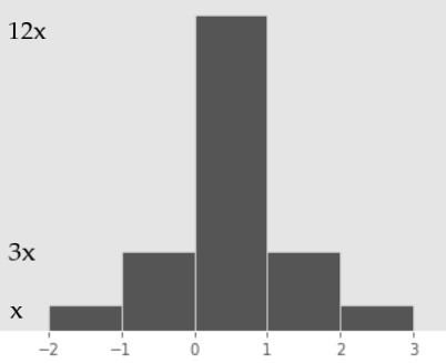
The heights of the five bars in this histogram, reading from left to right, are
x, 3x, 12x, 3x, x.
What is the value of x (i.e. the height of the shortest bar in the histogram)? Give your answer as a fully simplified fraction.
Answer: \frac{1}{20}
In any density histogram, the total area of all bars is 1. This histogram has five bars, each of which has a width of 1 (e.g. 3 - 2 = 1). Since \text{Area} = \text{Height} \cdot \text{Width}, we have that the area of each bar is equal to its height. So, the total area of the histogram in this case is the sum of the heights of each bar:
\text{Total Area} = x + 3x + 12x + 3x + x = 20x
Since we know that the total area is equal to 1, we have
20x = 1 \implies \boxed{x = \frac{1}{20}}
The average score on this problem was 72%.
What does the expression below evaluate to? Give your answer as an integer.
np.count_nonzero((sample_means > v2) & (sample_means <= v4))Hint: Don’t try to find the values of v2 and
v4 – you can answer this question without them!
Answer: 7,500
First, it’s a good idea to understand what the integer we’re trying
to find actually means in the context of the information provided. In
this case, it’s the number of sample means that are greater than
v2 and less than or equal to v4. Here’s how to
arrive at that conclusion:
sample_means is an array of length
10,000.sample_means > v2 and
sample_means <= v4 are both Boolean arrays of length
10,000.(sample_means > v2) & (sample_means <= v4) is
also a Boolean array of length 10,000, which contains True
for every sample mean that is greater than v2 and less than
or equal to v4 and False for every other
sample mean.np.count_nonzero((sample_means > v2) & (sample_means <= v4))
is a number between 0 and 10,000, corresponding to the
number of True elements in the array
(sample_means > v2) & (sample_means <= v4).Remember, the histogram we’re looking at visualizes the distribution
of the 10,000 values that result from calling f on every
value in sample_means. To proceed, we need to understand
how the function f decides what value to return
for a given input, v:
v is greater than v2, then
the first two conditions (v <= v1 and
v <= v2) are False, and so the only
possible values of f(v) are 0, 1,
or 2.v is less than or equal to
v4, the only possible values of f(v) are
-2, -1, 0, 1.v is greater than
v2 and less than or equal to v4, the
only possible values of f(v) are 0 and
1.Now, our job boils down to finding the number of values in the
visualized distribution that are equal to 0 or 1. This is equivalent to
finding the number of values that fall in the [0, 1) and [1,
2) bins – since f only returns integer values, the
only value in the [0, 1) bin is 0 and
the only value in the [1, 2) bin is 1
(remember, histogram bins are left-inclusive and right-exclusive).
To do this, we need to find the proportion of values in those two bins, and multiply that proportion by the total number of values (10,000).
We know that the area of a bar is equal to the proportion of values in that bin. We also know that, in this case, the area of each bar is equal to its height, since the width of each bin is 1. Thus, the proportion of values in a given bin is equal to the height of the corresponding bar. As such, the proportion of values in the [0, 1) bin is 12x, and the proportion of values in the [1, 2) bin is 3x, meaning the proportion of values in the histogram that are equal to either 0 or 1 is 12x + 3x = 15x.
In the previous subpart, we found that x = \frac{1}{20}, so the proportion of values in the histogram that are equal either 0 or 1 is 15 \cdot \frac{1}{20} = \frac{3}{4}*, and since there are 10,000 values being visualized in the histogram total, \frac{3}{4} \cdot 10,000 = 7,500 of them are equal to either 0 or 1.
Thus, 7,500 of the values in sample_means are greater
than v2 and less than or equal to v4, so
np.count_nonzero((sample_means > v2) & (sample_means <= v4))
evaluates to 7,500.
Note: It’s possible to answer this subpart without knowing the value of x, i.e. without answering the previous subpart. The area of the [0, 1) and [1, 2) bars is 15x, and the total area of the histogram is 20x. So, the proportion of the area in [0, 1) or [1, 2) is \frac{15x}{20x} = \frac{15}{20} = \frac{3}{4}, which is the same value we found by substituting x = \frac{1}{20} into 15x.
The average score on this problem was 40%.
Suppose we have run the code below.
from scipy import stats

def g(u):
    return stats.norm.cdf(u) - stats.norm.cdf(-u)
Several input-output pairs for the function g are shown
in the table below. Some of them will be useful to you in answering the
questions that follow.
u | g(u) |
|---|---|
| 0.84 | 0.60 |
| 1.28 | 0.80 |
| 1.65 | 0.90 |
| 2.25 | 0.975 |
What is the value of v3, one of the variables used in
the function f? Give your answer as a number.
Hint: Use the histogram as well as one of the rows of the table above.
Answer: 35.84
The table provided above tells us the proportion of values within u standard deviations of the mean in a normal distribution, for various values of u. For instance, it tells us that the proportion of values within 1.28 standard deviations of the mean in a normal distribution is 0.8.
Let’s reflect on what we know at the moment:
f returns 0 for all inputs that are
greater than v2 and less than or equal to v3.
This, combined with the fact above, tells us that the proportion
of sample means between v2 (exclusive) and v3
(inclusive) is 0.6.Combining the facts above, we have that v2 is 0.84
standard deviations below the mean of the sample mean’s distribution and
v3 is 0.84 standard deviations above the mean of the sample
mean’s distribution.
The sample mean’s distribution has the following characteristics:
\begin{align*} \text{Mean of Distribution of Possible Sample Means} &= \text{Population Mean} = 35 \\ \text{SD of Distribution of Possible Sample Means} &= \frac{\text{Population SD}}{\sqrt{\text{Sample Size}}} = \frac{10}{\sqrt{100}} = 1 \end{align*}
0.84 standard deviations above the mean of the sample mean’s distribution is:
35 + 0.84 \cdot \frac{10}{\sqrt{100}} = 35 + 0.84 \cdot 1 = \boxed{35.84}
So, the value of v3 is 35.84.
The average score on this problem was 9%.
Which of the following is closest to the value of the expression below?
np.percentile(sample_means, 5)14
14.75
33
33.35
33.72
Answer: 33.35
The table provided tells us that in a normal distribution, 90% of values are within 1.65 standard deviations of the mean. Since normal distributions are symmetric, it also means that 5% of values are above 1.65 standard deviations of the mean and, more importantly, 5% of values are below 1.65 standard deviations of the mean.
The 5th percentile of a distribution is the smallest value that is
greater than or equal to 5% of values, so in this case the 5th
percentile is 1.65 SDs below the mean. As in the previous subpart, the
mean and SD we are referring to are the mean and SD of the distribution
of sample means (sample_means), which we found to be 35 and
1, respectively.
1.65 standard deviations below this mean is
35 - 1.65 \cdot 1 = \boxed{33.35}
The average score on this problem was 45%.