← return to practice.dsc10.com
Instructor(s): Rod Albuyeh, Suraj Rampure, Janine Tiefenbruck
This exam was administered in-person. The exam was closed-notes, except students were provided a copy of the DSC 10 Reference Sheet. No calculators were allowed. Students had 3 hours to take this exam.
Note (groupby / pandas 2.0): Pandas 2.0+ no longer
silently drops columns that can’t be aggregated after a
groupby, so code written for older pandas may behave
differently or raise errors. In these practice materials we use
.get() to select the column(s) we want after
.groupby(...).mean() (or other aggregations) so that our
solutions run on current pandas. On real exams you will not be penalized
for omitting .get() when the old behavior would have
produced the same answer.
Today, we’re diving into the high-stakes world of fraud detection.
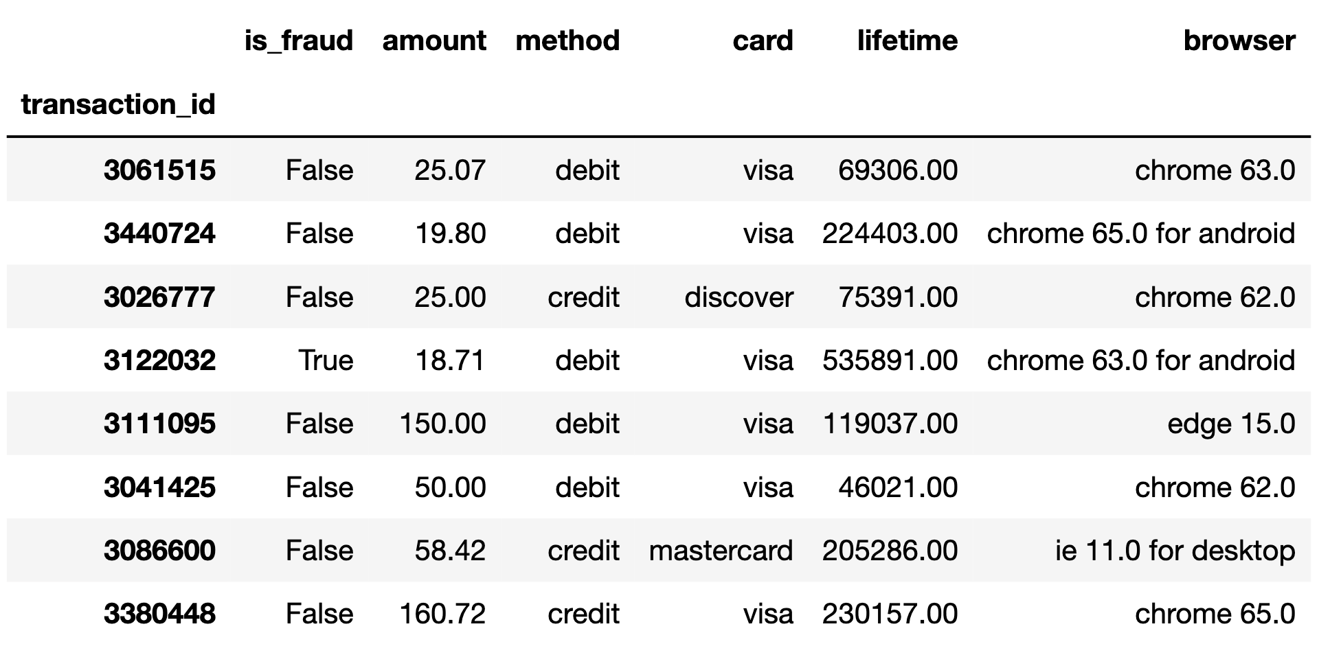
Each row in the DataFrame txn represents one online
transaction, or purchase. The txn DataFrame is indexed by
"transaction_id" (int), which is a unique identifier for a
transaction. The columns of txn are as follows:
"is_fraud" (bool): True if the transaction
was fraudulent and False if not."amount" (float): The dollar amount of the
transaction."method" (str): The payment method; either
"debit" or "credit"."card" (str): The payment network of the card used for
the transaction; either "visa", "mastercard",
"american express", or "discover"."lifetime" (float): The total transaction amount of all
transactions made with this card over its lifetime."browser" (str): The web browser used for the online
transaction. There are 100 distinct browser types in this column; some
examples include "samsung browser 6.2",
"mobile safari 11.0", and "chrome 62.0".The first few rows of txn are shown below, though
txn has 140,000 rows in total. Assume that the data in
txn is a simple random sample from the much larger
population of all online transactions.
Throughout this exam, assume that we have already run
import babypandas as bpd and
import numpy as np.
Nate’s favorite number is 5. He calls a number “lucky” if it’s
greater than 500 or if it contains a 5 anywhere in its representation.
For example, 1000.04 and 5.23 are both lucky
numbers.
Complete the implementation of the function check_lucky,
which takes in a number as a float and returns True if it
is lucky and False otherwise. Then, add a column named
"is_lucky" to txn that contains
True for lucky transaction amounts and False
for all other transaction amounts, and save the resulting DataFrame to
the variable luck.
        def check_lucky(x):
            return __(a)__

        luck = txn.assign(is_lucky = __(b)__)
What goes in blank (a)?
What goes in blank (b)?
Answer: (a):
x > 500 or "5" in str(x), (b):
txn.get("amount").apply(check_lucky)
(a): We want this function to return True if the number
is lucky (greater than 500 or if it has a 5 in it). Checking the first
condition is easy, we can simply use x > 500. To check the second
condition, we’ll convert the number to a string so that we can check
whether it contains "5" using the in keyword.
Once we have these two conditions written out, we can combine them with
the or keyword, since either one is enough for the number
to be considered lucky. This gives us the full statement
x > 500 or "5" in str(x). Since this will evaluate to
True if and only if the number is lucky, this is all we
need in the return statement.
The average score on this problem was 51%.
(b): Now that we have the is_lucky function, we want to
use it to find if each number in the amount column is lucky
or not. To do this, we can use .apply() to apply the
function elementwise (row-by-row) to the "amount" column,
which will create a new Series of Booleans indicating if each element in
the "amount" column is lucky.
The average score on this problem was 86%.
Fill in the blanks below so that lucky_prop evaluates to
the proportion of fraudulent "visa" card transactions whose
transaction amounts are lucky.
    visa_fraud = __(a)__
    lucky_prop = visa_fraud.__(b)__.mean()
What goes in blank (a)?
What goes in blank (b)?
Answer: (a):
luck[(luck.get("card")=="visa") & (luck.get("is_fraud"))],
(b): get("is_lucky")
(a): The first step in this question is to query the DataFrame so
that we have only the rows which are fraudulent transactions from “visa”
cards. luck.get("card")=="visa" evaluates to
True if and only if the transaction was from a Visa card,
so this is the first part of our condition. To find transactions which
were fraudulent, we can simply find the rows with a value of
True in the "is_fraud" column. We can do this
with luck.get("is_fraud"), which is equivalent to
luck.get("is_fraud") == True in this case since the
"is_fraud" column only contains Trues and Falses. Since we
want only the rows where both of these conditions hold, we can combine
these two conditions with the logical & operator, and
place this inside of square brackets to query the luck DataFrame for
only the rows where both conditions are true, giving us
luck[(luck.get("card")=="visa") & (luck.get("is fraud")].
Note that we use the & instead of the keyword
and since & is used for elementwise
comparisons between two Series, like we’re doing here, whereas the
and keyword is used for comparing two Booleans (not two
Series containing Booleans).
The average score on this problem was 52%.
(b): We already have a Boolean column is_lucky
indicating if each transaction had a lucky amount. Recall that booleans
are equivalent to 1s and 0s, where 1 represents true and 0 represents
false, so to find the proportion of lucky amounts we can simply take the
mean of the is_lucky column. The reason that taking the mean is
equivalent to finding the proportion of lucky amounts comes from the
definition of the mean: the sum of all values divided by the number of
entries. If all entries are ones and zeros, then summing the values is
equivalent to counting the number of ones (Trues) in the Series.
Therefore, the mean will be given by the number of Trues divided by the
length of the Series, which is exactly the proportion of lucky numbers
in the column.
The average score on this problem was 61%.
Fill in the blanks below so that lucky_prop is one value
in the Series many_props.
many_props = luck.groupby(__(a)__).mean().get(__(b)__)What goes in blank (a)?
What goes in blank (b)?
Answer: (a): [""card"", "is_fraud"],
(b): "is_lucky"
(a): lucky_prop is the proportion of fraudulent “visa”
card transactions that have a lucky amount. The idea is to create a
Series with the proportions of fraudulent or non-fraudulent transactions
from each card type that have a lucky amount. To do this, we’ll want to
group by the column that describes the card type ("card"),
and the column that describes whether a transaction is fraudulent
("is_fraud"). Putting this in the proper syntax for a
groupby with multiple columns, we have
["card", "is_fraud"]. The order doesn’t matter, so
["is_fraud", ""card""] is also correct.
The average score on this problem was 55%.
(b): Once we have this grouped DataFrame, we know that the entry in
each column will be the mean of that column for some combination of
"is_fraud" and "method". And, since
"is_lucky" contains Booleans, we know that this mean is
equivalent to the proportion of transactions which were lucky for each
"is_fraud" and "method" combination. One such
combination is fraudulent “visa” transactions, so
lucky_prop is one element of this Series.
The average score on this problem was 67%.
Consider the DataFrame combo, defined below.
combo = txn.groupby(["is_fraud", "method", "card"]).mean()What is the maximum possible value of combo.shape[0]?
Give your answer as an integer.
Answer: 16
combo.shape[0] will give us the number of rows of the
combo DataFrame. Since we’re grouping by
"is_fraud", "method", and "card",
we will have one row for each unique combination of values in these
columns. There are 2 possible values for "is_fraud", 2
possible values for "method", and 2 possible values for
"card", so the total number of possibilities is 2 * 2 * 4 =
16. This is the maximum number possible because 16 combinations of
"is_fraud", "method", and "card"
are possible, but they may not all exist in the data.
The average score on this problem was 75%.
What is the value of combo.shape[1]?
1
2
3
4
5
6
Answer: 2
combo.shape[1] will give us the number of columns of the
DataFrame. In this case, we’re using .mean() as our
aggregation function, so the resulting DataFrame will only have columns
with numeric types (since BabyPandas automatically ignores columns which
have a data type incompatible with the aggregation function). In this
case, "amount" and "lifetime" are the only
numeric columns, so combo will have 2 columns.
The average score on this problem was 47%.
Consider the variable is_fraud_mean, defined below.
is_fraud_mean = txn.get("is_fraud").mean()Which of the following expressions are equivalent to
is_fraud_mean? Select all that apply.
txn.groupby("is_fraud").mean()
txn.get("is_fraud").sum() / txn.shape[0]
np.count_nonzero(txn.get("is_fraud")) / txn.shape[0]
(txn.get("is_fraud") > 0.8).mean()
1 - (txn.get("is_fraud") == 0).mean()
None of the above.
Answer: B, C, D, and E.
The correct responses are B, C, D, and E. First, we must see that
txn.get("is_fraud").mean() will calculate the mean of the
"is_fraud" column, which is a float representing the
proportion of values in the "is_fraud" column that are
True. With this in mind, we can consider each option:
Option A: This operation will result in a DataFrame. We first
group by "is_fraud", creating one row for fraudulent
transactions and one row for non-fraudulent ones. We then take the mean
of each numerical column, which will determine the entries of the
DataFrame. Since this results in a DataFrame and not a float, this
answer choice cannot be correct.
Option B: Here we simply take the mean of the
"is_fraud" column using the definition of the mean as the
sum of the values divided by the nuber of values. This is equivalent to
the original.
Option C: np.count_nonzero will return the number of
nonzero values in a sequence. Since we only have True and False values
in the "is_fraud" column, and Python considers
True to be 1 and False to be 0, this means
counting the number of ones is equivalent to the sum of all the values.
So, we end up with an expression equivalent to the formula for the mean
which we saw in part B.
Option D: Recall that "is_fraud" contains Boolean
values, and that True evaluates to 1 and False
evaluates to 0. txn.get("is_fraud") > 0.8 conducts an
elementwise comparison, evaluating if each value in the column is
greater than 0.8, and returning the resulting Series of Booleans. Any
True (1) value in the column will be greater than 0.8, so
this expression will evaluate to True. Any
False (0) value will still evaluate to False,
so the values in the resulting Series will be identical to the original
column. Therefore, taking the mean of either will give the same
value.
Option E: txn.get("is_fraud") == 0 performs an
elementwise comparison, returning a series which has the value
True where "is_fraud" is False
(0), and False where "is_fraud" is
True. Therefore the mean of this Series represents the
proportion of values in the "is_fraud" column that are
False. Since every value in that column is either
False or True, the proportion of
True values is equivalent to one minus the proportion of
False values.
The average score on this problem was 69%.
The following code block produces a bar chart, which is shown directly beneath it.
    (txn.groupby("browser").mean()
        .sort_values(by="is_fraud", ascending=False)
        .take(np.arange(10))
        .plot(kind="barh", y="is_fraud"))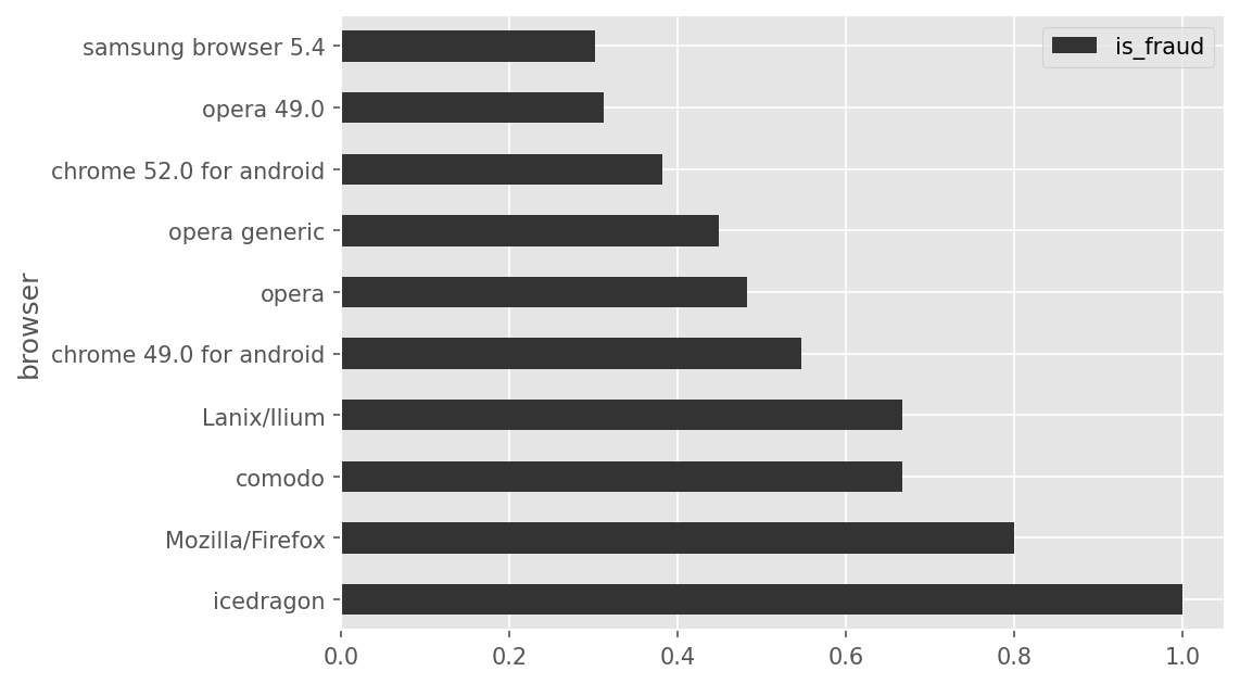
Based on the above bar chart, what can we conclude about the browser
"icedragon"? Select all that apply.
In our dataset, "icedragon" is the most frequently used
browser among all transactions.
In our dataset, "icedragon" is the most frequently used
browser among fraudulent transactions.
In our dataset, every transaction made with "icedragon"
is fraudulent.
In our dataset, there are more fraudulent transactions made with
"icedragon" than with any other browser.
None of the above.
Answer: C
First, let’s take a look at what the code is doing. We start by
grouping by browser and taking the mean, so each column will have the
average value of that column for each browser (where each browser is a
row). We then sort in descending order by the "is_fraud"
column, so the browser which has the highest proportion of fraudulent
transactions will be first, and we take first the ten browsers, or those
with the most fraud. Finally, we plot the "is_fraud" column
in a horizontal bar chart. So, our plot shows the proportion of
fraudulent transactions for each browser, and we see that
icedragon has a proportion of 1.0, implying that every
transaction is fraudulent. This makes the third option correct. Since we
don’t have enough information to conclude any of the other options, the
third option is the only correct one.
The average score on this problem was 83%.
How can we modify the provided code block so that the bar chart displays the same information, but with the bars sorted in the opposite order (i.e. with the longest bar at the top)?
Change ascending=False to
ascending=True.
Add .sort_values(by="is_fraud", ascending=True)
immediately before .take(np.arange(10)).
Add .sort_values(by="is_fraud", ascending=True)
immediately after .take(np.arange(10)).
None of the above.
Answer: C
Let’s analyze each option A: This isn’t correct, because we must
remember that np.take(np.arange(10)) takes the rows indexed
0 through 10. And if we change ascending = False to
ascending = True, the rows indexed 0 through 10 won’t be
the same in the resulting DataFrame (since now they’ll be the 10
browsers with the lowest fraud rate). B: This will have
the same effect as option A, since it’s being applied before the
np.take() operation C: Once we have the 10 rows with the
highest fraud rate, we can sort them in ascending order in order to
reverse the order of the bars. Since we already have the 10 rows from
the original plot, this option is correct.
The average score on this problem was 59%.
The DataFrame seven, shown below to the
left, consists of a simple random sample of 7 rows from
txn, with just the "is_fraud" and
"amount" columns selected.
The DataFrame locations, shown below to the
right, is missing some values in its
"is_fraud" column.
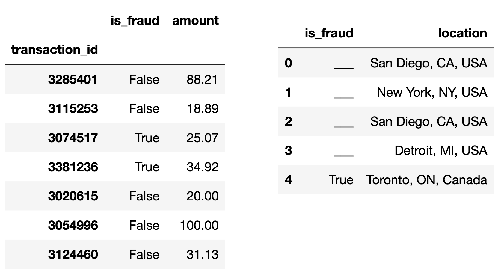
Fill in the blanks to complete the "is_fraud" column of
locations so that the DataFrame
seven.merge(locations, on="is_fraud") has
19 rows.
Answer A correct answer has one True
and three False rows.
We’re merging on the "is_fraud" column, so we want to
look at which rows have which values for "is_fraud". There
are only two possible values (True and False),
and we see that there are two Trues and 5
Falses in seven. Now, think about what happens
“under the hood” for this merge, and how many rows are created when it
occurs. Python will match each True in seven
with each True in the "is_fraud" column of
location, and make a new row for each such pair. For
example, since Toronto’s row in location has a
True value in location, the merged DataFrame
will have one row where Toronto is matched with the transaction of
$34.92 and one where Toronto is matched with the transaction of $25.07.
More broadly, each True in locations creates 2
rows in the merged DataFrame, and each False in
locations creates 5 rows in the merged DataFrame. The
question now boils down to creating 19 by summing 2s and 5s. Notice that
19 = 3\cdot5+2\cdot2. This means we can
achieve the desired 19 rows by making sure the locations
DataFrame has three False rows and two True
rows. Since location already has one True, we
can fill in the remaining spots with three Falses and one
True. It doesn’t matter which rows we make
True and which ones we make False, since
either way the merge will produce the same number of rows for each (5
each for every False and 2 each for every
True).
The average score on this problem was 88%.
True or False: It is possible to fill in the four blanks in the
"is_fraud" column of locations so that the
DataFrame seven.merge(locations, on="is_fraud") has
14 rows.
True
False
Answer: False
As we discovered by solving problem 5.1, each False
value in locations gives rise to 5 rows of the merged
DataFrame, and each True value gives rise to 2 rows. This
means that the number of rows in the merged DataFrame will be m\cdot5 + n\cdot2, where m is the number of
Falses in location and n is the number of
Trues in location. Namely, m and n are
integers that add up to 5. There’s only a few possibilities so we can
try them all, and see that none add up 14:
0\cdot5 + 5\cdot2 = 10
1\cdot5 + 4\cdot2 = 13
2\cdot5 + 3\cdot2 = 16
3\cdot5 + 2\cdot2 = 19
4\cdot5 + 1\cdot2 = 22
The average score on this problem was 79%.
Aaron wants to explore the discrepancy in fraud rates between
"discover" transactions and "mastercard"
transactions. To do so, he creates the DataFrame ds_mc,
which only contains the rows in txn corresponding to
"mastercard" or "discover" transactions.
After he creates ds_mc, Aaron groups ds_mc
on the "card" column using two different aggregation
methods. The relevant columns in the resulting DataFrames are shown
below.
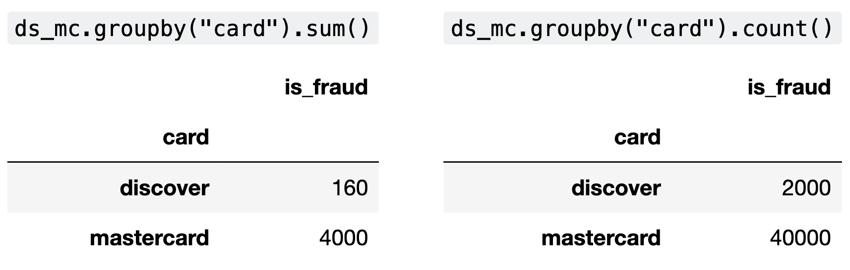
Aaron decides to perform a test of the following pair of hypotheses:
Null Hypothesis: The proportion of fraudulent
"mastercard" transactions is the same as
the proportion of fraudulent "discover"
transactions.
Alternative Hypothesis: The proportion of
fraudulent "mastercard" transactions is less
than the proportion of fraudulent "discover"
transactions.
As his test statistic, Aaron chooses the difference in
proportion of transactions that are fraudulent, in the order
"mastercard" minus "discover".
What type of statistical test is Aaron performing?
Standard hypothesis test
Permutation test
Answer: Permutation test
Permutation tests are used to ascertain whether two samples were
drawn from the same population. Hypothesis testing is used when we have
a single sample and a known population, and want to determine whether
the sample appears to have been drawn from that population. Here, we
have two samples (“mastercard” and “discover”)
and no known population distribution, so a permutation test is the
appropriate test.
The average score on this problem was 49%.
What is the value of the observed statistic? Give your answer either as an exact decimal or simplified fraction.
Answer: 0.02
We simply take the difference in fraudulent proportion of
"mastercard" transactions and fraudulent proportion of
discover transactions. There are 4,000 fraudulent
"mastercard" transactions and 40,000 total
"mastercard" transactions, making this proportion for
"mastercard". Similarly, the proportion of fraudulent
"discover" transactions is \frac{160}{2000}. Simplifying these
fractions, the difference between them is \frac{1}{10} - \frac{8}{100} = 0.1 - 0.08 =
0.02.
The average score on this problem was 86%.
The empirical distribution of Aaron’s chosen test statistic is shown below.
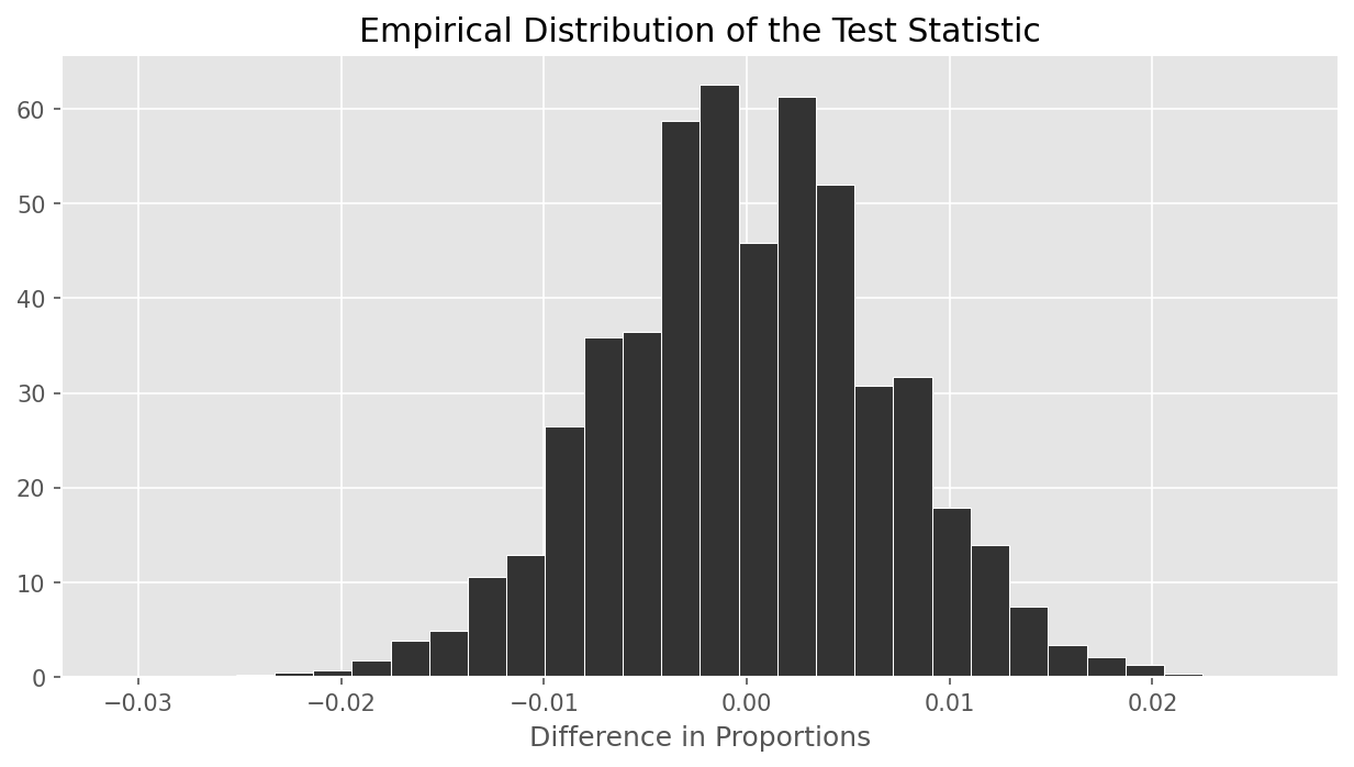
Which of the following is closest to the p-value of Aaron’s test?
0.001
0.37
0.63
0.94
0.999
Answer: 0.999
Informally, the p-value is the area of the histogram at or past the
observed statistic, further in the direction of the alternative
hypothesis. In this case, the alternative hypothesis is that the
"mastercard" proportion is less than the discover
proportion, and our test statistic is computed in the order
"mastercard" minus "discover", so low
(negative) values correspond to the alternative. This means when
calculating the p-value, we look at the area to the left of 0.02 (the
observed value). We see that essentially all of the test statistics fall
to the left of this value, so the p-value should be closest to
0.999.
The average score on this problem was 54%.
What is the conclusion of Aaron’s test?
The proportion of fraudulent "mastercard" transactions
is less than the proportion of fraudulent
"discover" transactions.
The proportion of fraudulent "mastercard" transactions
is greater than the proportion of fraudulent
"discover" transactions.
The test results are inconclusive.
None of the above.
Answer: None of the above
"mastercard" transactions is less
than the proportion of fraudulent "discover" transactions,
so we cannot conclude A.
The average score on this problem was 44%.
Aaron now decides to test a slightly different pair of hypotheses.
Null Hypothesis: The proportion of fraudulent
"mastercard" transactions is the same as
the proportion of fraudulent "discover"
transactions.
Alternative Hypothesis: The proportion of
fraudulent "mastercard" transactions is greater
than the proportion of fraudulent "discover"
transactions.
He uses the same test statistic as before.
Which of the following is closest to the p-value of Aaron’s new test?
0.001
0.06
0.37
0.63
0.94
0.999
Answer: 0.001
Now, we have switched the alternative hypothesis to “
"mastercard" fraud rate is greater than
"discover" fraud rate”, whereas before our alternative
hypothesis was that the "mastercard" fraud rate was less
than "discover"’s fraud rate. We have not changed the way
we calculate the test statistic ("mastercard" minus
"discover"), so now large values of the test statistic
correspond to the alternative hypothesis. So, the area of interest is
the area to the right of 0.02, which is very small, close to 0.001. Note
that this is one minus the p-value we computed before.
The average score on this problem was 65%.
Jason is interested in exploring the relationship between the browser
and payment method used for a transaction. To do so, he uses
txn to create create three tables, each of which contain
the distribution of browsers used for credit card transactions and the
distribution of browsers used for debit card transactions, but with
different combinations of browsers combined in a single category in each
table.
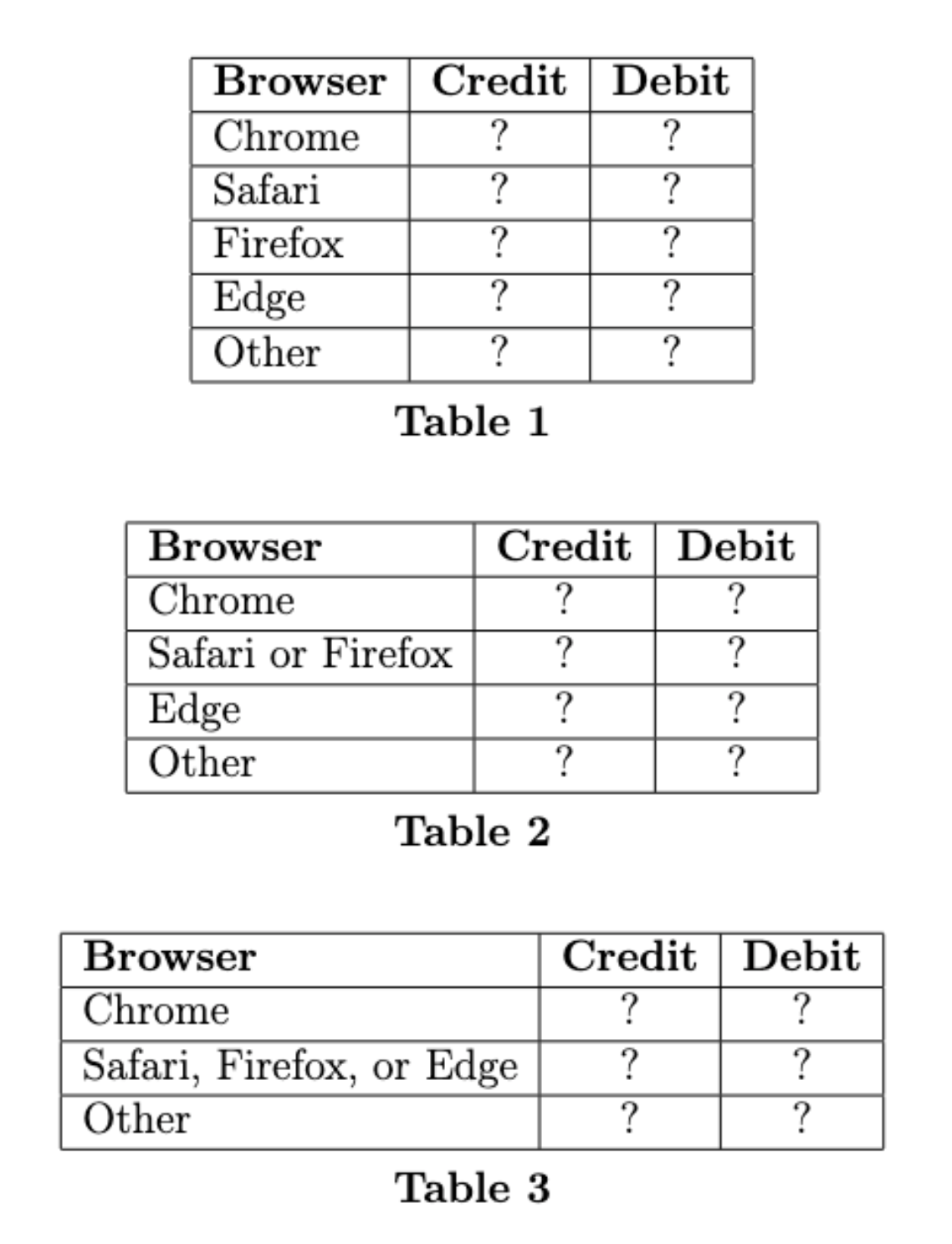
Jason calculates the total variation distance (TVD) between the two distributions in each of his three tables, but he does not record which TVD goes with which table. He computed TVDs of 0.14, 0.36, and 0.38.
In which table do the two distributions have a TVD of 0.14?
Table 1
Table 2
Table 3
Answer: Table 3
Without values in any of the tables, there’s no way to do this problem computationally. We are told that the three TVDs come out to 0.14, 0.36, and 0.38. The exact numbers are not important but their relative order is. The key to this problem is noticing that when we combine two categories into one, the TVD can only decrease, it cannot increase. One way to see this is to think about combining categories repeatedly until there’s just one category. Then both distributions must have a value of 1 in that category so they are identical distributions with the smallest possible TVD of 0. As we collapse categories, we can only decrease the TVD. This tells us that Table 1 has the largest TVD, then Table 2 has the middle TVD, and Table 3 has the smallest, since each time we are combining categories and shrinking the TVD.
The average score on this problem was 77%.
In which table do the two distributions have a TVD of 0.36?
Table 1
Table 2
Table 3
Answer: Table 2
See the solution to 7.1.
The average score on this problem was 97%.
In which table do the two distributions have a TVD of 0.38?
Table 1
Table 2
Table 3
Answer: Table 1
See the solution to 7.1.
The average score on this problem was 77%.
Since txn has 140,000 rows, Jack wants to get a quick
glimpse at the data by looking at a simple random sample of 10 rows from
txn. He defines the DataFrame ten_txns as
follows:
ten_txns = txn.sample(10, replace=False)Which of the following code blocks also assign ten_txns
to a simple random sample of 10 rows from txn?
Option 1:
    all_rows = np.arange(txn.shape[0])
    perm = np.random.permutation(all_rows)
    positions = np.random.choice(perm, size=10, replace=False)
    ten_txn = txn.take(positions)
Option 2:
    all_rows = np.arange(txn.shape[0])
    choice = np.random.choice(all_rows, size=10, replace=False)
    positions = np.random.permutation(choice)
    ten_txn = txn.take(positions)
Option 3:
    all_rows = np.arange(txn.shape[0])
    positions = np.random.permutation(all_rows).take(np.arange(10))
    ten_txn = txn.take(positions)
Option 4:
    all_rows = np.arange(txn.shape[0])
    positions = np.random.permutation(all_rows.take(np.arange(10)))
    ten_txn = txn.take(positions)
Select all that apply.
Option 1
Option 2
Option 3
Option 4
None of the above.
Answer: Option 1, Option 2, and Option 3.
Let’s consider each option.
Option 1: First, all_rows is defined as an array
containing the integer positions of all the rows in the DataFrame. Then,
we randomly shuffle the elements in this array and store it in the array
permutations. Finally, we select 10 integers randomly
(without replacement), and use .take() to select the rows
from the DataFrame with the corresponding integer locations. In other
words, we are randomly selecting ten row numbers and taking those
randomly selected. This gives a simple random sample of 10 rows from the
DataFrame txn, so option 1 is correct.
Option 2: Option 2 is similar to option 1, except that the order
of the np.random.choice and the
np.random.permutation operations are switched. This doesn’t
affect the output, since the choice we made was, by definition, random.
Therefore, it doesn’t matter if we shuffle the rows before or after (or
not at all), since the most this will do is change the order of a sample
which was already randomly selected. So, option 2 is correct.
Option 3: Here, we randomly shuffle the elements of
all_rows, and then we select the first 10 elements with
np.take. Since the shuffling of elements from
all_rows was random, we don’t know which elements are in
the first 10 positions of this new shuffled array (in other words, the
first 10 elements are random). So, when we select the rows from
txn which have the corresponding integer locations in the
next step, we’ve simply selected 10 rows with random integer locations.
Therefore, this is a valid random sample from txn, and
option 3 is correct.
Option 4: The difference between this option and option 3 is the
order in which np.random.permutation and
np.take are executed. Here, we select the first 10 elements
before the permutation (inside the parentheses). As a result, the array
which we’re shuffling with np.random.permutation does not
include all the integer locations like all_rows does, it’s
simply the first ten elements. Therefore, this code produces a random
shuffling of the first 10 rows of txn, which is not a
random sample.
The average score on this problem was 82%.
The DataFrame ten_txns, displayed in its
entirety below, contains a simple random sample of 10 rows from
txn.
Suppose we randomly select one transaction from
ten_txns. What is the probability that the selected
transaction is made with a "card" of
"mastercard" or a "method" of
"debit"? Give your answer either as an exact decimal or a
simplified fraction.
Answer: 0.7
We can simply count the number of transactions meeting at least one
of the two criteria. More easily, there are only 3 rows that do not meet
either of the criteria (the rows that are "visa" and
"credit" transactions). Therefore, the probability is 7 out
of 10, or 0.7. Note that we cannot simply add up the probability of
"mastercard" (0.3) and the probability of
"debit" (0.6) since there is overlap between these. That
is, some transactions are both "mastercard" and
"debit".
The average score on this problem was 64%.
Suppose we randomly select two transactions from
"ten_txns", without replacement, and learn that neither of
the selected transactions is for an amount of 100 dollars. Given this
information, what is the probability that:
the first transaction is made with a "card" of
"visa" and a "method" of "debit",
and
the second transaction is made with a "card" of
"visa" and a "method" of
"credit"?
Give your answer either as an exact decimal or a simplified fraction.
Answer: \frac{2}{15}
We know that the sample space here doesn’t have any of the $100
transactions, so we can ignore the first 4 rows when calculating the
probability. In the remaining 6 rows, there are exactly 2 debit
transactions with "visa" cards, so the probability of our
first transaction being of the specified type is \frac{2}{6}. There are also two credit
transactions with "visa" cards, but the denominator of the
probability of the second transaction is 5 (not 6), since the sample
space was reduced by one after the first transaction. We’re choosing
without replacement, so you can’t have the same transaction in your
sample twice. Thus, the probability of the second transaction being a
visa credit card is \frac{2}{5}. Now,
we can apply the multiplication rule, and we have that the probability
of both transactions being as described is \frac{2}{6} \cdot \frac{2}{5} = \frac{4}{30} =
\frac{2}{15}.
The average score on this problem was 45%.
For your convenience, we show ten_txns again below.
Suppose we randomly select 15 rows, with replacement, from
ten_txns. What’s the probability that in our selection of
15 rows, the maximum transaction amount is less than 25 dollars?
\frac{3}{10}
\frac{3}{15}
\left(\frac{3}{10}\right)^{3}
\left(\frac{3}{15}\right)^{3}
\left(\frac{3}{10}\right)^{10}
\left(\frac{3}{15}\right)^{10}
\left(\frac{3}{10}\right)^{15}
\left(\frac{3}{15}\right)^{15}
Answer: \left(\frac{3}{10}\right)^{15}
There are only 3 rows in the sample with a transaction amount under $25, so the chance of choosing one transaction with such a low value is \frac{3}{10}. For the maximum transaction amount to be less than 25 dollars, this means all transaction amounts in our sample have to be less than 25 dollars. To find the chance that all transactions are for less than $25, we can apply the multiplication rule and multiply the probability of each of the 15 transactions being less than $25. Since we’re choosing 15 times with replacement, the events are independent (choosing a certain transaction on the first try won’t affect the probability of choosing it again later), so all the terms in our product are \frac{3}{10}. Thus, the probability is \frac{3}{10} * \frac{3}{10} * \ldots * \frac{3}{10} = \left(\frac{3}{10}\right)^{15}.
The average score on this problem was 89%.
As a senior suffering from senioritis, Weiyue has plenty of time on his hands. 1,000 times, he repeats the following process, creating 1,000 confidence intervals:
Collect a simple random sample of 100 rows from
txn.
Resample from his sample 10,000 times, computing the mean transaction amount in each resample.
Create a 95% confidence interval by taking the middle 95% of resample means.
He then computes the width of each confidence interval by subtracting its left endpoint from its right endpoint; e.g. if [2, 5] is a confidence interval, its width is 3. This gives him 1,000 widths. Let M be the mean of these 1,000 widths.
Select the true statement below.
About 950 of Weiyue’s intervals will contain the mean transaction amount of all transactions ever.
About 950 of Weiyue’s intervals will contain the mean transaction
amount of all transactions in txn.
About 950 of Weiyue’s intervals will contain the mean transaction
amount of all transactions in the first random sample of 100 rows of
txn Weiyue took.
About 950 of Weiyue’s intervals will contain M.
Answer: About 950 of Weiyue’s intervals will contain
the mean transaction amount of all transactions in txn.
By the definition of a 95% confidence interval, 95% of our 1000
confidence intervals will contain the true mean transaction amount in
the population from which our samples were drawn. In this case, the
population is the txn DataFrame. So, 950 of the confidence
intervals will contain the mean transaction amount of all transactions
in txn, which is what the the second answer choice
says.
We can’t conclude that the first answer choice is correct because our
original sample was taken from txn, not from all
transactions ever. We don’t know whether our resamples will be
representative of all transactions ever. The third option is incorrect
because we have no way of knowing what the first random sample looks
like from a statistical standpoint. The last statement is not true
because M concerns the width of the
confidence interval, and therefore is unrelated to the statistics
computed in each resample. For example, if the mean of each resample is
around 100, but the width of each confidence interval is around 5, we
shouldn’t expect $$M to be in any of the confidence intervals.
The average score on this problem was 55%.
Weiyue repeats his entire process, except this time, he changes his sample size in step 1 from 100 to 400. Let B be the mean of the widths of the 1,000 new confidence intervals he creates.
What is the relationship between M and B?
M < B
M \approx B
M > B
Answer: M > B
As the sample size increases, the width of the confidence intervals will decrease, so M > B.
The average score on this problem was 70%.
Weiyue repeats his entire process once again. This time, he still uses a sample size of 100 in step 1, but instead of creating 95% confidence intervals in step 3, he creates 99% confidence intervals. Let C be the mean of the widths of the 1,000 new confidence intervals he generates.
What is the relationship between M and C?
M < C
M \approx C
M > C
Answer: M < C
All else equal (note that the sample size is the same as it was in question 10.1), 99% confidence intervals will always be wider than 95% confidence intervals on the same data, so M < C.
The average score on this problem was 85%.
Weiyue repeats his entire process one last time. This time, he still uses a sample size of 100 in step 1, and creates 95% confidence intervals in step 3, but instead of bootstrapping, he uses the Central Limit Theorem to generate his confidence intervals. Let D be the mean of the widths of the 1,000 new confidence intervals he creates.
What is the relationship between M and D?
M < D
M \approx D
M > D
Answer: M \approx D
Confidence intervals generated from the Central Limit Theorem will be approximately the same as those generated from bootstrapping, so M is approximately equal to D.
The average score on this problem was 90%.
On Reddit, Yutian read that 22% of all online transactions are fraudulent. She decides to test the following hypotheses:
Null Hypothesis: The proportion of online transactions that are fraudulent is 0.22.
Alternative Hypothesis: The proportion of online transactions that are fraudulent is not 0.22.
To test her hypotheses, she decides to create a 95% confidence interval for the proportion of online transactions that are fraudulent using the Central Limit Theorem.
Unfortunately, she doesn’t have access to the entire txn
DataFrame; rather, she has access to a simple random sample of
txn of size n. In her
sample, the proportion of transactions that are fraudulent is
0.2 (or equivalently, \frac{1}{5}).
The width of Yutian’s confidence interval is of the form \frac{c}{5 \sqrt{n}}
where n is the size of her sample and c is some positive integer. What is the value of c? Give your answer as an integer.
Hint: Use the fact that in a collection of 0s and 1s, if the proportion of values that are 1 is p, the standard deviation of the collection is \sqrt{p(1-p)}.
Answer: 8
First, we can calculate the standard deviation of the sample using the given formula: \sqrt{0.2\cdot(1-0.2)} = \sqrt{0.16}= 0.4. Additionally, we know that the width of a 95% confidence interval for a population mean (including a proportion) is approximately \frac{4 * \text{sample SD}}{\sqrt{n}}, since 95% of the data of a normal distribution falls within two standard deviations of the mean on either side. Now, plugging the sample standard deviation into this formula, we can set this expression equal to the given formula for the width of the confidence interval: \frac{c}{5 \sqrt{n}} = \frac{4 * 0.4}{\sqrt{n}}. We can multiply both sides by \sqrt{n}, and we’re left with \frac{c}{5} = 4 * 0.4. Now, all we have to do is solve for c by multiplying both sides by 5, which gives c = 8.
The average score on this problem was 59%.
There is a positive integer J such that:
If n < J, Yutian will fail to reject her null hypothesis at the 0.05 significance level.
If n > J, Yutian will reject her null hypothesis at the 0.05 significance level.
What is the value of J? Give your answer as an integer.
Answer: 1600
Here, we have to use the formula for the endpoints of the 95% confidence interval to see what the largest value of n is such that 0.22 will be contained in the interval. The endpoints are given by \text{sample mean} \pm 2 * \frac{\text{sample SD}}{\sqrt{n}}. Since the null hypothesis is that the proportion is 0.22 (which is greater than our sample mean), we only need to work with the right endpoint for this question. Plugging in the values that we have, the right endpoint is given by 0.2 + 2 * \frac{0.4}{\sqrt{n}}. Now we must find a value of n which satisfies the inequality 0.2 + 2 * \frac{0.4}{\sqrt{n}} \geq 0.22, and since we’re looking for the smallest such value of n (i.e, the last n for which this inequality holds), we can simply set the two sides equal to each other, and solve for n. From 0.2 + 2 * \frac{0.4}{\sqrt{n}} = 0.22, we can subtract 0.2 from both sides, then multiply both sides by \sqrt{n}, and divide both sides by 0.02 (from 0.22 - 0.2). This yields \sqrt{n} = \frac{2 * 0.4}{0.02} = \sqrt{n} = 40, which implies that n is 1600.
The average score on this problem was 21%.
On Reddit, Keenan also read that 22% of all online transactions are fraudulent. He decides to test the following hypotheses at the 0.16 significance level:
Null Hypothesis: The proportion of online transactions that are fraudulent is 0.22.
Alternative Hypothesis: The proportion of online transactions that are fraudulent is not 0.22.
Keenan has access to a simple random sample of txn of
size 500. In his sample, the proportion of transactions
that are fraudulent is 0.23.
Below is an incomplete implementation of the function
reject_null, which creates a bootstrap-based confidence
interval and returns True if the conclusion of Keenan’s
test is to reject the null hypothesis, and
False if the conclusion is to fail to
reject the null hypothesis, all at the 0.16
significance level.
    def reject_null():
        fraud_counts = np.array([])
        for i in np.arange(10000):
            fraud_count = np.random.multinomial(500, __(a)__)[0]
            fraud_counts = np.append(fraud_counts, fraud_count)

        L = np.percentile(fraud_counts, __(b)__)
        R = np.percentile(fraud_counts, __(c)__)

        if __(d)__ < L or __(d)__ > R:
            # Return True if we REJECT the null.
            return True
        else:
            # Return False if we FAIL to reject the null.
            return False
Fill in the blanks so that reject_null works as
intended.
Hint: Your answer to (d) should be an integer greater than 50.
Answer:
[0.23, 0.77]892110(a): Because we’re bootstrapping, we’re using the data from the
original sample. This is not a “regular” hypothesis testing where we
simulate under the assumptions of the null. It’s more like the human
body temperature example from lecture, where are constructing a
confidence interval, then we’ll determine which hypothesis to side with
based on whether some value falls in the interval or not. Here, they
tell us to make a bootstrapped confidence interval. Normally we’d use
the .sample method for this, but we’re forced here to use
np.random.multinomial, which also works because that
samples with replacement from a categorical distribution, and since
we’re working with a dataset of just two values for whether a
transaction is fraudulent or not, we can think of resampling from our
original sample as drawing from a categorical distribution.
We know that the proportion of fraudulent transactions in the sample
is 0.23 (and therefore the non-fraudulent proportion is 0.77), so we use
these as the probabilities for np.random.multinomial in our
bootstrapping simulation. The syntax for this function requires us to
pass in the probabilities as a list, so the answer is
[0.23, 0.77].
The average score on this problem was 23%.
(b): Since we’re testing at the 0.16 significance level, we know that
the proportion of data lying outside either of our endpoints is 0.16, or
0.08 on each side. So, the left endpoint is given by the 8th percentile,
which means that the argument to np.percentile must be
8.
The average score on this problem was 67%.
(c): Similar to part B, we know that 0.08 of the data must lie to the
right of the right endpoint, so the argument to
np.percentile here is (1 - 0.08)
\cdot 100 = 92.
The average score on this problem was 67%.
(d): To test our hypothesis, we must compare the left and right endpoints to the observed value. If the observed value is less than the left endpoint or greater than the right endpoint, we will reject the null hypothesis. Otherwise we fail to reject it. Since the left and right endpoints give the count of fraudulent transactions (not the proportion), we must convert our null hypothesis to similar terms. We can simply multiply the sample size by the proportion of fraudulent transactions to obtain the count that the null hypothesis would suggest given the sample size of 500, which gives us 500 * 0.22 = 110.
The average score on this problem was 26%.
Ashley doesn’t have access to the entire txn DataFrame;
instead, she has access to a simple random sample of
400 rows of txn.
She draws two histograms, each of which depicts the distribution of
the "amount" column in her sample, using different
bins.
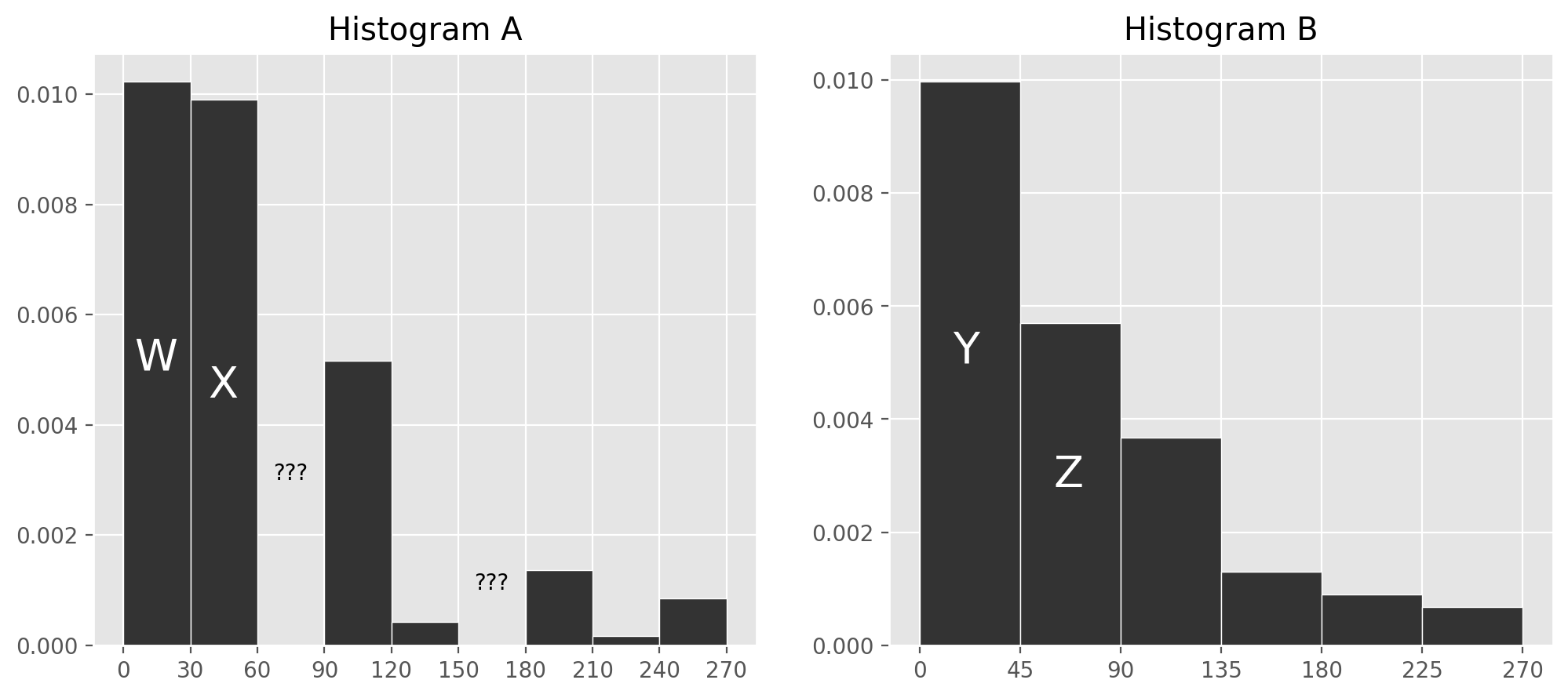
Unfortunately, DataHub is being finicky and so two of the bars in Histogram A are deleted after it is created.
In Histogram A, which of the following bins contains approximately 60 transactions?
[30, 60)
[90, 120)
[120, 150)
[180, 210)
Answer: [90, 120)
The number of transactions contained in the bin is given by the area of the bin times the total number of transactions, since the area of a bin represents the proportion of transactions that are contained in that bin. We are asked which bin contains about 60 transactions, or \frac{60}{400} = \frac{3}{20} = 0.15 proportion of the total area. All the bins in Histogram A have a width of 30, so for the area to be 0.15, we need the height h to satisfy h\cdot 30 = 0.15. This means h = \frac{0.15}{30} = 0.005. The bin [90, 120) is closest to this height.
The average score on this problem was 90%.
Let w, x, y, and z be the heights of bars W, X, Y, and Z, respectively. For instance, y is about 0.01.
Which of the following expressions gives the height of the bar corresponding to the [60, 90) bin in Histogram A?
( y + z ) - ( w + x )
( w + x ) - ( y + z )
\frac{3}{2}( y + z ) - ( w + x )
( y + z ) - \frac{3}{2}( w + x )
3( y + z ) - 2( w + x )
2( y + z ) - 3( w + x )
None of the above.
Answer: \frac{3}{2}( y + z ) - ( w + x )
The idea is that the first three bars in Histogram A represent the same set of transactions as the first three bars of Histogram B. Setting these areas equals gives 30w+30x+30u= 45y+45z, where u is the unknown height of the bar corresponding to the [60, 90) bin. Solving this equation for u gives the result.
\begin{align*} 30w+30x+30u &= 45y+45z \\ 30u &= 45y+45z-30w-30x \\ u &= \frac{45y + 45z - 30w - 30x}{30} \\ u &= \frac{3}{2}(y+z) - (w+x) \end{align*}
The average score on this problem was 50%.
As mentioned in the previous problem, Ashley has sample of 400 rows
of txn. Coincidentally, in Ashley’s sample of 400
transactions, the mean and standard deviation of the
"amount" column both come out to 70 dollars.
Fill in the blank:
“According to Chebyshev’s inequality, at most 25 transactions in
Ashley’s sample
are above ____ dollars; the rest must be below ____ dollars."
What goes in the blank? Give your answer as an integer. Both blanks are filled in with the same number.
Answer: 350
Chebyshev’s inequality says something about how much data falls within a given number of standard deviations. The data that doesn’t fall in that range could be entirely below that range, entirely above that range, or split some below and some above. So the idea is that we should figure out the endpoints of the range for which Chebyshev guarantees that at least 375 transactions must fall. Then at most 25 might fall above that range. So we’ll fill in the blank with the upper limit of that range. Now, since there are 400 transactions, 375 as a proportion becomes \frac{375}{400} = \frac{15}{16}. That’s 1 - \frac{1}{16} or 1 - \left(\frac{1}{4}\right)^2, so we should use z=4 in the statement of Chebyshev’s inequality. That is, \frac{15}{16} proportion of the data falls within 4 standard deviations of the mean. The upper endpoint of that range is 70 (the mean) plus 4 \cdot 70 (four standard deviations), or 5 \cdot 70 = 350.
The average score on this problem was 30%.
Now, we’re given that the mean and standard deviation of the
"lifetime" column in Ashley’s sample are both equal to
c dollars. We’re also given that the
correlation between transaction amounts and lifetime spending in
Ashley’s sample is -\frac{1}{4}.
Which of the four options could be a scatter plot of lifetime spending vs. transaction amount?
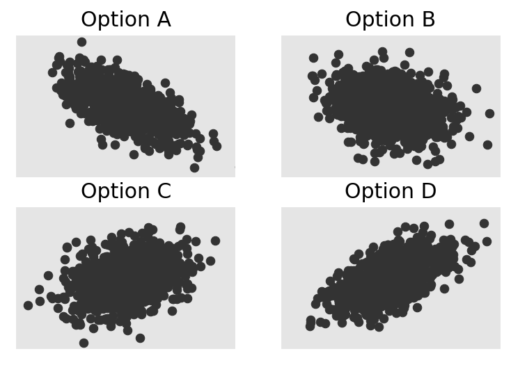
Option A
Option B
Option C
Option D
Answer: Option B
Here, the main factor which we can use to identify the correct plot is the correlation coefficient. A correlation coefficient of -\frac{1}{4} indicates that the data will have a slight downward trend (values on the y axis will be lower as we go further right). This narrows it down to option A or option B, but option A appears to have too strong of a linear trend. We want the data to look more like a cloud than a line since the correlation is relatively close to zero, which suggests that option B is the more viable choice.
The average score on this problem was 89%.
Ashley decides to use linear regression to predict the lifetime spending of a card given a transaction amount.
The predicted lifetime spending, in dollars, of a card with a transaction amount of 280 dollars is of the form f \cdot c, where f is a fraction. What is the value of f? Give your answer as a simplified fraction.
Answer: f = \frac{1}{4}
This problem requires us to make a prediction using the regression line for a given x = 280. We can solve this problem using original units or standard units. Since 280 is a multiple of 70, and the mean and standard deviation are both 70, it’s pretty straightforward to convert 280 to 3 standard units, as \frac{(280-70)}{70} = \frac{210}{70} = 3. To make a prediction in standard units, all we need to do is multiply by r=-\frac{1}{4}, resulting in a predicted lifetime spending of =-\frac{3}{4} in standard units. Since we are told in the previous subpart that both the mean and standard deviation of lifetime spending are c dollars, then converting to original units gives c + -\frac{3}{4} \cdot c = \frac{1}{4} \cdot c, so f = \frac{1}{4}.
The average score on this problem was 42%.
Suppose the intercept of the regression line, when both transaction amounts and lifetime spending are measured in dollars, is 40. What is the value of c? Give your answer as an integer.
Answer: c = 32
We start with the formulas for the mean and intercept of the regression line, then set the mean and SD of x both to 70, and the mean and SD of y both to c, as well as the intercept b to 40. Then we can solve for c.
\begin{align*} m &= r \cdot \frac{\text{SD of } y}{\text{SD of }x} \\ b &= \text{mean of } y - m \cdot \text{mean of } x \\ m &= -\frac{1}{4} \cdot \frac{c}{70} \\ 40 &= c - (-\frac{1}{4} \cdot \frac{c}{70}) \cdot 70 \\ 40 &= c + \frac{1}{4} c \\ 40 &= \frac{5}{4} c \\ c &= 40 \cdot \frac{4}{5} \\ c &= 32 \end{align*}
The average score on this problem was 45%.