← return to practice.dsc10.com
Instructor(s): Janine Tiefenbruck
This exam was administered in-person. The exam was closed-notes, except students were allowed to bring one sheet of handwritten notes. No calculators were allowed. Students had 3 hours to take this exam.
⚠️ PDF version available here .
Note (groupby / pandas 2.0): Pandas 2.0+ no longer
silently drops columns that can’t be aggregated after a
groupby, so code written for older pandas may behave
differently or raise errors. In these practice materials we use
.get() to select the column(s) we want after
.groupby(...).mean() (or other aggregations) so that our
solutions run on current pandas. On real exams you will not be penalized
for omitting .get() when the old behavior would have
produced the same answer.
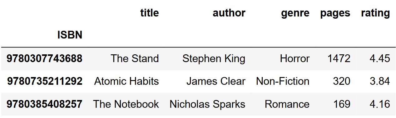
Bill has opened a bookstore, called Bill’s Book Bonanza. In the
DataFrame bookstore, each row corresponds to a unique book
available at this bookstore. The index is "ISBN"
(int), which is a unique identifier for books. The columns
are:
"title" (str): The title of the book."author" (str): The author of the
book."genre" (str): The primary genre of the
book."pages" (int): The number of pages in the
book."rating" (float): The rating of the book,
out of 5 stars. This data comes from Goodreads, a book review
website.The first three rows are shown below, though bookstore
has many more rows than pictured.
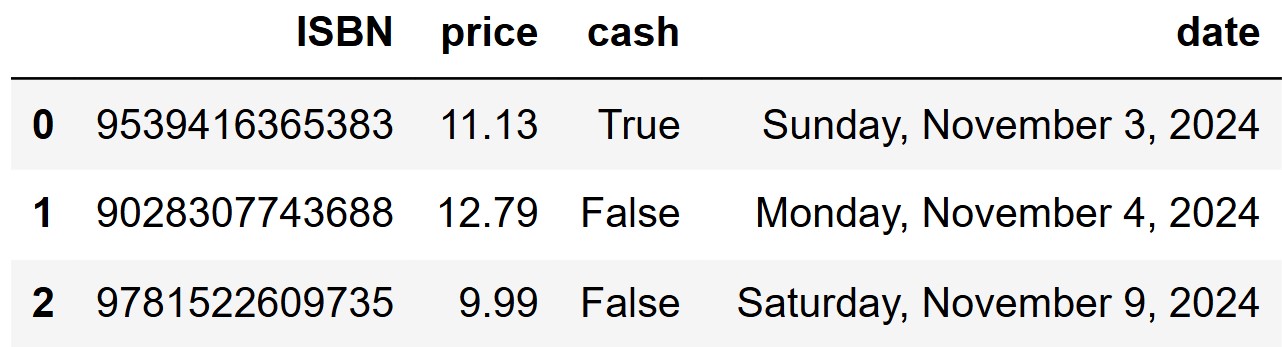
Additionally, we are given a dataset of sales, which
lists all the book purchases made from Bill’s Book Bonanza since it
opened. The columns of sales are:
"ISBN" (str): The unique identifier for
the book."price" (float): The price of the book at
Bill’s Book Bonanza."cash" (bool): True if the
purchase was made in cash and False if not."date" (str): The date the book purchase
was made, using the format
"Day of the Week, Month Day, Year". See below for
examples.The first three rows of sales are shown below, though
sales has many more rows than this.
Throughout this exam, we will refer to bookstore and
sales repeatedly.
Assume that we have already run
import babypandas as bpd, import numpy as np,
and import scipy.
Notice that bookstore has an index of
"ISBN" and sales does not. Why is that?
There is no good reason. We could have set the index of
sales to "ISBN".
There can be two different books with the same
"ISBN".
"ISBN" is already being used as the index of
bookstore, so it shouldn’t also be used as the index of
sales.
The bookstore can sell multiple copies of the same book.
Answer: The bookstore can sell multiple copies of the same book.
In the sales DataFrame, each row represents an
individual sale, meaning multiple rows can have the same
"ISBN" if multiple copies of the same book are sold.
Therefore we can’t use it as the index because it is not a unique
identifier for rows of sales.
The average score on this problem was 87%.
Is "ISBN" a numerical or categorical variable?
numerical
categorical
Answer: categorical
Even though "ISBN" consists of numbers, it is used to
identify and categorize books rather than to quantify or measure
anything, thus it is categorical. It doesn’t make sense to compare ISBN
numbers like you would compare numbers on a number line, or to do
arithmetic with ISBN numbers.
The average score on this problem was 75%.
Which type of data visualization should be used to compare authors by median rating?
scatter plot
line plot
bar chart
histogram
Answer: bar chart
A bar chart is best, as it visualizes numerical values (median ratings) across discrete categories (authors).
The average score on this problem was 88%.
ISBN numbers for books must follow a very particular format. The first 12 digits encode a lot of information about a book, including the publisher, edition, and physical properties like page count. The 13th and final digit, however, is computed directly from the first 12 digits and is used to verify that a given ISBN number is valid.
In this question, we will define a function to compute the final digit of an ISBN number, given the first 12. First, we need to understand how the last digit is determined. To find the last digit of an ISBN number:
Multiply the first digit by 1, the second digit by 3, the third digit by 1, the fourth digit by 3, and so on, alternating 1s and 3s.
Add up these products.
Find the ones digit of this sum.
If the ones digit of the sum is zero, the final digit of the ISBN is zero. Otherwise, the final digit of the ISBN is ten minus the ones digit of the sum.
For example, suppose we have an ISBN number whose first 12 digits are 978186197271. Then the last digit would be calculated as follows: 9\cdot 1 + 7\cdot 3 + 8\cdot 1 + 1\cdot 3 + 8\cdot 1 + 6\cdot 3 + 1\cdot 1 + 9\cdot 3 + 7\cdot 1 + 2\cdot 3 + 7\cdot 1 + 1\cdot 3 = 118 The ones digit is 8 so the final digit is 2.
Fill in the blanks in the function calculate_last_digit
below. This function takes as input a string
representing the first 12 digits of the ISBN number, and should return
the final digit of the ISBN number, as an int. For example,
calculate_last_digit("978186197271") should evaluate to
2.
def calculate_last_digit(partial_isbn_string):
    total = 0
    for i in __(a)__:
        digit = int(partial_isbn_string[i])
        if __(b)__:
            total = total + digit
        else:
            total = total + 3 * digit
    ones_digit = __(c)__
    if __(d)__:
        return 10 - ones_digit
return 0Note: this procedure may seem complicated, but it is actually how the last digit of an ISBN number is generated in real life!
np.arange(12) or np.arange(len(partial_isbn_string))We need to loop through all of the digits in the partial string we are given.
The average score on this problem was 62%.
i % 2 == 0 or i in [0, 2, 4, 6, 8, 10]If we are at an even position, we want to add the digit itself (or the digit times 1). We can check if we are at an even positon by checking the remainder upon division by 2, which is 0 for all even numbers and 1 for all odd numbers.
The average score on this problem was 41%.
total % 10 or int(str(total)[-1])We need the ones digit of the total to determine what to return. We
can treat total as an integer and get the ones digit by
finding the remainder upon division by 10, or we can convert
total to a string, extract the last character with
[-1], and then convert back to an int.
The average score on this problem was 44%.
ones_digit != 0In most cases, we subtract the ones digit from 10 and return that. If the ones digit is 0, we just return 0.
The average score on this problem was 87%.
At the beginning of 2025, avid reader Michelle will join the Blind Date with a Book program sponsored by Bill’s Book Bonanza. Once a month from January through December, Michelle will receive a surprise book in the mail from the bookstore. So she’ll get 12 books throughout the year.
Each book is randomly chosen among those available at the bookstore
(or equivalently, from among those in the bookstore
DataFrame). Each book is equally likely to be chosen each month, and
each month’s book is chosen independently of all others, so repeats can
occur.
Let p be the proportion of books in
bookstore from the romance genre (0 \leq p \leq 1).
What is the probability that the books Michelle receives in February and December are romance, while the books she receives all other months are non-romance? Your answer should be an unsimplified expression in terms of p.
Answer: (1 - p)^{10} * p^2
The probability of February and December being romance is p for each of those two months, and the probability of any one of the other months being non-romance is 1-p. We multiply all twelve of these probabilities since the months are independent, and the result is p^2(1−p)^{10}.
The average score on this problem was 57%.
What is the probability that at least one of the books Michelle receives in the last four months of the year is romance? Your answer should be an unsimplified expression in terms of p.
Answer: 1 - (1 - p)^4
To solve this, we calculate the probability that none of the last four months contains romance, which is (1−p)^4. Taking the complement gives us the probability that at least one of the last four months is romance: 1−(1−p)^4. The two possible situations are: no romance and at least one romance, so together they must add up to one, which is why we can use the complement.
The average score on this problem was 51%.
It is likely Michelle will receive at least one romance book and at least one non-romance book throughout the 12 months of the year. What is the probability that this does not happen? Your answer should be an unsimplified expression in terms of p.
Answer: p^{12} + (1 - p)^{12}
In this case, there are only two scenarios to consider: either all 12 books are non-romance, which gives (1−p)^{12}, or all 12 books are romance, which gives p^{12}. Adding these together gives p^{12}+(1−p)^{12}.
The average score on this problem was 29%.
Let n be the total number of rows in
bookstore. What is the probability that Michelle does not
receive any duplicate books in the first four months of the year? Your
answer should be an unsimplified expression in terms of n.
Answer: \frac{(n - 1)}{n} * \frac{(n - 2)}{n} * \frac{(n - 3)}{n}
For there to be no duplicate books in the first four months, each subsequent book must be different from the previous ones. After selecting the first book (which will always be undiplicated), the second book has \frac{(n - 1)}{n} probability of being unique, the third \frac{(n - 2)}{n}, and the fourth \frac{(n - 3)}{n}. If you like, you can think of the probability of the first book being unique as \frac{n}{n} and include it in your answer.
The average score on this problem was 31%.
Now, consider the following lines of code which define variables
i, j, and k.
    def foo(x, y):
        if x == "rating":
            z = bookstore[bookstore.get(x) > y]
        elif x == "genre":
            z = bookstore[bookstore.get(x) == y]
        return z.shape[0]

    i = foo("rating", 3)
    j = foo("rating", 4)
    k = foo("genre", "Romance")
For both questions that follow, your answer should be an unsimplified
expression in terms of i, j, k
only. If you do not have enough information to determine the answer,
leave the answer box blank and instead fill in the bubble that says “Not
enough information”.
If we know in advance that Michelle’s January book will have a rating greater than 3, what is the probability that the book’s rating is greater than 4?
Answer: j/i
Looking at the code, we can see that i represents the
number of books with a rating greater than 3, and j
represents the number of books with a rating greater than 4. This is a
conditional probability question: find the probability that Michelle’s
book has a rating greater than 4 given that it has a rating greater than
3. Since we already know Michelle’s book has a rating higher than 3, the
denominator, representing the possible books she could get, should be
i. The numerator represents the books that meet our desired
condition of having a rating greater than 4, which is j.
Therefore, the result is j/i.
The average score on this problem was 53%.
If we know in advance that Michelle’s January book will have a rating greater than 3, what is the probability that the book’s genre is romance?
Although i represents the total number of books with a
rating greater than 3 and k represents the number of
romance books, there is no information about how many romance books have
a rating greater than 3. Thus we cannot find the answer without
additional information.
The average score on this problem was 71%.
Matilda has been working at Bill’s Book Bonanza since it first opened
and her shifts for each week are always randomly scheduled (i.e., she
does not work the same shifts each week). Due to the system restrictions
at the bookstore, when Matilda logs in with her employee ID, she only
has access to the history of sales made during her shifts. Suppose these
transactions are stored in a DataFrame called matilda,
which has the same columns as the sales DataFrame that
stores all transactions.
Matilda wants to use her random sample to estimate the mean
price of books purchased with cash at Bill’s Book Bonanza. For
the purposes of this question, assume Matilda only has access to
matilda, and not all of sales.
Complete the code below so that cash_left and
cash_right store the endpoints of an 86\% bootstrapped confidence interval for the
mean price of books purchased with cash at Bill’s Book Bonanza.
    cash_means = np.array([])
    original = __(a)__
    for i in np.arange(10000):
        resample = original.sample(__(b)__)
        cash_means = np.append(cash_means, __(c)__)

    cash_left = __(d)__
cash_right = __(e)__matilda[matilda.get("cash")]We first filter the matilda DataFrame to only include
rows where the payment method was cash, since these are the only rows
that are relevant to our question of the mean price of books purchased
with cash.
The average score on this problem was 65%.
original.shape[0], replace = TrueWe repeatedly resample from this filtered data. We always bootstrap using the same sample size as the original sample, and with replacement.
The average score on this problem was 79%.
resample.get("price").mean()Our statistic is the mean price, which we need to calculate from the
resample DataFrame.
The average score on this problem was 71%.
np.percentile(cash_means, 7)Since our goal is to construct an 86% confidence interval, we take the 7^{th} percentile as the left endpoint and the 93^{rd} percentile as the right endpoint. These numbers come from 100 - 86 = 14, which means we want 14\% of the area excluded from our interval, and we want to split that up evenly with 7\% on each side.
The average score on this problem was 84%.
np.percentile(cash_means, 93)
The average score on this problem was 84%.
Next, Matilda uses the data in matilda to construct a
95\% CLT-based confidence interval for
the same parameter.
Given that there are 400 cash transactions in matilda
and her confidence interval comes out as [19.58, 21.58], what is the standard
deviation of the prices of all cash transactions at Bill’s Book
Bonanza?
Answer: 10
The width of the interval is 21.58 - 19.58 = 2. Using the formula for the width of a 95\% CLT-based confidence interval and solving for the standard deviation gives the answer.
Width = 4 * \frac{SD}{\sqrt{400}}
SD = 2 * \frac{\sqrt{400}}{4} = 10
The average score on this problem was 61%.
Knowing the endpoints of Matilda’s 95% CLT-based confidence interval can actually help us to determine the endpoints of her 86% bootstrapped confidence interval. You may also need to know the following facts:
stats.norm.cdf(1.1) evaluates to
0.86
stats.norm.cdf(1.5) evaluates to
0.93
Estimate the value of cash_left to one decimal
place.
Answer: 19.8
The useful fact here is the second fact. It says that if you step 1.5 standard deviations to the right of the mean in a normal distribution, 93% of the area will be to the left. Since that leaves 7% of the area to the right, this also means that the area to the left of -1.5 standard units is 7%, by symmetry. So the area between -1.5 and 1.5 standard units is 86% of the area, or the bounds for an 86% confidence interval. This is the grey area in the picture below.
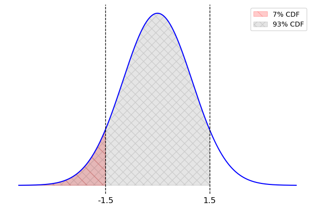
The middle of our interval is 20.58 so we calculate the left endpoint as:
\begin{align*} \texttt{cash\_left} &= 20.58 - 1.5 * \frac{SD}{\sqrt{n}}\\ &= 20.58 - 1.5 * \frac{10}{\sqrt{400}}\\ &= 20.58 - 0.75 \\ &= 19.83\\ &\approx 19.8 \end{align*}
The average score on this problem was 22%.
Which of the following are valid conclusions? Select all that apply.
Approximately 95% of the values in cash_means fall
within the interval [19.58, 21.58].
Approximately 95% of books purchased with cash at Bill’s Book Bonanza have a price that falls within the interval [19.58, 21.58].
The actual mean price of books purchased with cash at Bill’s Book Bonanza has a 95% chance of falling within the interval [19.58, 21.58].
None of the above.
Answer: Approximately 95% of the values in
cash_means fall within the interval [19.58, 21.58].
Choice 1 is correct because of the way bootstrapped confidence
intervals are created. If we made a 95% bootstrapped confidence interval
from cash_means, it would capture 95% of the values in cash_means,
by design. This is not how the interval [19.58, 21.58] was created, however; this
interval comes from the CLT. However bootstrapped and CLT-based
confidence intervals give very nearly the same results. They are two
methods to solve the same problem and they create nearly identical
confidence intervals. So it is correct to say that approximately 95% of
the values in cash_means fall within a 95% CLT-based
confidence interval, which is [19.58,
21.58].
Choice 2 is incorrect because the interval estimates the mean price, not individual book prices.
Choice 3 is incorrect because confidence intervals are about the reliability of the method: if we repeated the whole bootstrapping process many times, about 95% of the intervals would contain the true mean. It does not indicate the probability of the true mean being within this specific interval because this interval is fixed and the true mean is also fixed. It doesn’t make sense to talk about the probability of a fixed number falling in a fixed interval; that’s like asking if there’s a 95% chance that 5 is between 2 and 10.
The average score on this problem was 63%.
Matilda has been wondering whether the mean price of books purchased with cash at Bill’s Book Bonanza is \$20. What can she conclude about this?
The mean price of books purchased with cash at Bill’s Book Bonanza is $20.
The mean price of books purchased with cash at Bill’s Book Bonanza could plausibly be $20.
The mean price of books purchased with cash at Bill’s Book Bonanza is not $20.
The mean price of books purchased with cash at Bill’s Book Bonanza is most likely not $20.
Answer: The mean price of books purchased with cash at Bill’s Book Bonanza could plausibly be $20.
This question is referring to a hypothesis test where we test whether parameter (in this case, the mean price of books purchased with cash) is equal to a specific value ($20). The hypothesis test can be conducted by constructing a confidence interval for the parameter and checking whether the specific value falls in the interval. Since $20 is within the confidence interval, it is a plausible value for the parameter, but never guaranteed.
The average score on this problem was 90%.
Aathi is a movie enthusiast looking to dive into book-reading. He visits Bill’s Book Bonanza and asks for help from the employee on duty, Matilda.
Matilda has access to the matilda DataFrame of
transactions from her shifts, as well as the bookstore
DataFrame of all books available in the store. She decides to advise
Aathi based on the ratings of books that are popular enough to have been
purchased during her shifts. Unfortunately, matilda does
not contain information about the rating or genre of the books sold. To
fix this, she merges the two DataFrames and keeps only the columns that
she’ll need.
Fill in the blanks in the code below so that the resulting
merged DataFrame has one row for each book in
matilda, and columns representing the genre and rating of
each such book.
merged = (matilda.merge(bookstore, __(a)__, __(b)__)
.get(["genre", "rating"]))left_on = "ISBN"
right_index = True
Since each "ISBN" uniquely identifies a book, we can
merge on that. We use right_index=True because
"ISBN" is the index in bookstore, not a
column. We need to match it with the "ISBN" column in
matilda.
The average score on this problem was 60%.
In this example, matilda and merged have
the same number of rows. Why is this the case? Choose the answer which
is sufficient alone to guarantee the same number of rows.
Because every book in bookstore appears exactly once in
matilda.
Because every book in matilda appears exactly once in
bookstore.
Because matilda has no duplicate rows.
Because bookstore has no duplicate rows.
Because the books in matilda are a subset of the books
in bookstore.
Answer: Because every book in matilda
appears exactly once in bookstore.
Think about the merging process. Imagine we go through each row of
matilda, one row at a time, and look for corresponding rows
that match in bookstore. If each row of
matilda matches with exactly one row of
bookstore, then the merged DataFrame must have the same
number of rows as matilda started with.
The average score on this problem was 53%.
Matilda uses some babypandas operations on the
merged DataFrame to create the DataFrame pictured below,
which she calls top_two.
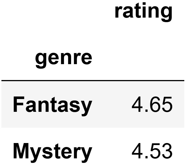
This DataFrame shows the two genres in merged with the
highest mean rating. Note that the "rating" column in
top_two represents a mean rating across many books of the
same genre, not the rating of any individual book.
Write one line of code to define the DataFrame top_two
as described above. It’s okay if you need to write your answer on
multiple lines, as long as it represents one line of code.
Answer:
top_two = merged.groupby("genre").mean().sort_values(by="rating", ascending=False).take([0, 1])
We first groupby the merged DataFrame by
"genre" and calculates the mean rating for each genre. Then
we sort these genres by their average rating in descending order so the
higest rated are at the top. Finally, we select the top two genres with
the highest average ratings using .take([0, 1]), which
keeps only the first two rows.
The average score on this problem was 67%.
Based on the data in top_two, Matilda recommends that
Aathi purchase a fantasy book. However, Aathi is skeptical because he
recognizes that the data in merged is only a sample from
the larger population of all transactions at Bill’s Book Bonanza. Before
he makes his purchase, he decides to do a permutation test to determine
whether fantasy books have higher ratings than mystery books in this
larger population.
Select the best statement of the null hypothesis for this permutation test.
Among all books sold at Bill’s Book Bonanza, fantasy books have a higher rating than mystery books, on average.
Among all books sold at Bill’s Book Bonanza, fantasy books do not have a higher rating than mystery books, on average.
Among all books sold at Bill’s Book Bonanza, fantasy books have the same rating as mystery books, on average.
Answer: Among all books sold at Bill’s Book Bonanza, fantasy books have the same rating as mystery books, on average.
The null hypothesis for a permutation test assumes that there is no difference in the population means, implying that fantasy and mystery books have the same average ratings.
The average score on this problem was 62%.
Select the best statement of the alternative hypothesis for this permutation test.
Among all books sold at Bill’s Book Bonanza, fantasy books have a higher rating than mystery books, on average.
Among all books sold at Bill’s Book Bonanza, fantasy books do not have a higher rating than mystery books, on average.
Among all books sold at Bill’s Book Bonanza, fantasy books have the same rating as mystery books, on average.
Answer: Among all books sold at Bill’s Book Bonanza, fantasy books have a higher rating than mystery books, on average.
The alternative hypothesis is that that fantasy books have higher ratings than mystery books, representing the claim being tested against the null hypothesis.
The average score on this problem was 69%.
Aathi decides to use the mean rating for mystery books minus the mean rating for fantasy books as his test statistic. What is his observed value of this statistic?
Answer: -0.12
This comes from subtracting the values provided in the grouped DataFrame in the order mystery minus fantasy: 4.53 - 4.65 = -0.12.
The average score on this problem was 80%.
Which of the following best describes how Aathi will interpret the results of his permutation test?
High values of the observed statistic will make him lean towards the alternative hypothesis.
Low values of the observed statistic will make him lean towards the alternative hypothesis.
Both high and low values of the observed statistic will make him lean towards the alternative hypothesis.
Answer: Low values of the observed statistic will make him lean towards the alternative hypothesis.
Since we are subtracting in the order mystery rating minus fantasy rating, a low (negative) observed statistic would indicate that fantasy books have higher ratings than mystery books. So low values would cause us to reject the null in favor of the alternative.
The average score on this problem was 66%.
Fill in the blanks in the following code to perform Aathi’s permutation test.
just_two = merged[(merged.get("genre") == "Fantasy") |
                  (merged.get("genre") == "Mystery")]

rating_stats = np.array([])
for i in np.arange(10000):
    shuffled = just_two.assign(shuffled = __(a)__)
    grouped = shuffled.groupby("genre").mean().get("shuffled")
    mystery_mean = grouped.iloc[__(b)__]
    fantasy_mean = grouped.iloc[__(c)__]
rating_stats = np.append(rating_stats, mystery_mean - fantasy_mean)np.random.permutation(just_two.get("rating"))We have to permute the "rating" column because of the
code provided on the next line, which groups by genre.
The average score on this problem was 75%.
1It’s important for this question to know that
.groupby("genre") sorts genres alphabetically. In this case, the genre“Fantasy”is before“Mystery”alphabetically,“Mystery”corresponds to the second row (iloc[1]`).
The average score on this problem was 57%.
0 The average score on this problem was 60%.
"Fantasy" is located in the first row, so we use
iloc[0].
Aathi gets a p_value of 0.008, and he will base his purchase on this
result, using the standard p-value cutoff of 0.05. What will Aathi end up doing?
Aathi fails to reject the null hypothesis and will purchase a fantasy book.
Aathi fails to reject the null hypothesis and will purchase a mystery book.
Aathi rejects the null hypothesis and will purchase a fantasy book.
Aathi rejects the null hypothesis and will purchase a mystery book.
Answer: Aathi rejects the null hypothesis and will purchase a fantasy book.
The p-value is lower than our cutoff of 0.05 so we reject the null hypothesis because our observed data doesn’t look like the data we simulated under the assumptions of the null hypothesis.
The average score on this problem was 68%.
Bill is curious about whether his bookstore is busier on weekends (Saturday, Sunday) or weekdays (Monday, Tuesday, Wednesday, Thursday, Friday). To help figure this out, he wants to define some helpful one-line functions.
The function find_day should take in a given
"date" and return the associated day of the week. For
example, find_day("Saturday, December 7, 2024") should
evaluate to "Saturday".
The function is_weekend should take in a given
"date" and return True if that date is on a
Saturday or Sunday, and False otherwise. For example,
is_weekend("Saturday, December 7, 2024") should evaluate to
True.
Complete the implementation of both functions below.
def find_day(date):
    return date.__(a)__

def weekend(date):
return find_day(date)[__(b)__] == __(c)__(a). Answer: split(",")[0]
The function find_day takes in a string that is a date
with the format "Day of week, Month Day, Year", and we want
the "Day of week" part. .split(",") separates
the given string by "," and gives us a list containing the
separated substrings, which looks something like
["Saturday", " December 7", " 2024"]. We want the first
element in the list, so we use [0] to obtain the first
element of the list.
The average score on this problem was 89%.
(b). Answer: 0
This blank follows a call of find_day(date), which
returns a string that is a day of the week, such as
"Saturday". The blank is inside a pair of [],
hinting that we are performing string indexing to pull out a specific
character from the string. We want to determine whether the string is
"Saturday" or "Sunday". The only thing in
common for these two days and is not common for the other five days of
the week is that the string starts with the letter "S".
Thus, we get the first character using [0] in this
blank.
The average score on this problem was 74%.
(c). Answer: "S"
After getting the first character in the string, to check whether it
is the letter "S", we use == to evaluate this
character against "S". This expression will give us a
boolean, either True or False, which is then
returned.
The average score on this problem was 50%.
Now, Bill runs the following line of code:
sales_day = sales.assign(weekend = sales.get("date").apply(is_weekend))Determine which of the following code snippets evaluates to the
proportion of book purchases in sales that were made on a
weekend. Select all that apply.
sales_day[sales_day.get("weekend")].count() / sales_day.shape[0]
sales[sales_day.get("weekend")].shape[0] / sales_day.shape[0]
sales_day.get("weekend").median()
sales_day.get("weekend").mean()
np.count_nonzero(sales_day.get("weekend") > 0.5) / sales_day.shape[0]
Answer:
sales[sales_day.get("weekend")].shape[0] / sales_day.shape[0]sales_day.get("weekend").mean()np.count_nonzero(sales_day.get("weekend") > 0.5) / sales_day.shape[0]First of all, we add a new column called "weekend" to
the sales DataFrame, and this new DataFrame is called
sales_day. The new column contains boolean values that
indicate whether the value in the "date" column is
"Saturday" or "Sunday", which are obtained by
applying is_weekend from the previous question to the
"date" column.
Now, we want to find the proportion of book purchases in sales that
were made on a weekend, which is basically the proportion of rows in the
"weekend" column that are True. Let’s look at
each of the options:
sales_day[sales_day.get("weekend")].count() / sales_day.shape[0]
(incorrect): You can only use .count() on a groupby object.
The correct alternative is to use .shape[0].
sales[sales_day.get("weekend")].shape[0] / sales_day.shape[0]
(correct): sales_day.get("weekend") gets the
"weekend column from the sales_day DataFrame.
We then use this Series to query the sales DataFrame and
keep only the rows corresponding to weekends. Lastly, we count the
number of rows in this filtered DataFrame with .shape[0]
and divide by the total number of sales to get the proportion.
sales_day.get("weekend").median() (incorrect): A
boolean value can be seen as 1 (True) or 0 (False). Since the column
"weekend" contains all booleans, the median falls on either
1 or 0, which is not the proportion that we want.
sales_day.get("weekend").mean() (correct): A boolean
value can be seen as 1 (True) or 0 (False). The mean of the
"weekend" column is equal to the sum of the column divided
the total number of rows in the column. The sum of the column is the sum
of all the 1’s and 0’s, which is just the number of Trues.
The number of Trues divided by the total number of rows is
the proportion of sales on weekend.
np.count_nonzero(sales_day.get("weekend") > 0.5) / sales_day.shape[0]
(correct): A boolean value can be seen as 1 (True) or 0 (False).
sales_day.get("weekend") > 0.5 gives us a Series of
booleans indicating whether the value in "weekend" is
greater than 0.5. If the value is True, then it’s greater
than 0.5. np.count_nonzero counts the number of values that
are not zero, which is the number of Trues. We then divide
the number of Trues by the total number of sales to get the
proportion.
The average score on this problem was 72%.
Hargen is an employee at Bill’s Book Bonanza who tends to work weekend shifts. He thinks that Fridays, Saturdays, and Sundays are busier than other days, and he proposes the following probability distribution of sales by day:
| Sunday | Monday | Tuesday | Wednesday | Thursday | Friday | Saturday |
|---|---|---|---|---|---|---|
| 0.2 | 0.1 | 0.1 | 0.1 | 0.1 | 0.2 | 0.2 |
Let’s use the data in sales to determine whether
Hargen’s proposed model could be correct by doing a hypothesis test. The
hypotheses are:
Null Hypothesis: Sales at the bookstore are randomly drawn from Hargen’s proposed distribution of days.
Alternative Hypothesis: Sales at the bookstore are not randomly drawn from Hargen’s proposed distribution of days.
Which of the following test statistics could be used to test the given hypothesis? Select all that apply.
The absolute difference between the proportion of books sold on Saturday and the proposed proportion of books sold on Saturday (0.2).
The sum of the differences in proportions between the distribution of books sold by day and Hargen’s proposed distribution.
The sum of the squared differences in proportions between the distribution of books sold by day and Hargen’s proposed distribution.
One half of the sum of the absolute differences in proportions between the distribution of books sold by day and Hargen’s proposed distribution.
Answer:
Let’s look at each of the options:
The average score on this problem was 74%.
We will use as our test statistic the mean of the absolute differences in proportions between the distribution of books sold by day and Hargen’s proposed distribution.
Suppose the observed distribution of books sold by day was as follows. Calculate the observed statistic in this case.
| Sunday | Monday | Tuesday | Wednesday | Thursday | Friday | Saturday |
|---|---|---|---|---|---|---|
| 0.34 | 0.13 | 0.06 | 0.07 | 0.08 | 0.08 | 0.24 |
Answer: 0.06
\begin{align*} \text{mean abs diff} &= \frac{|0.34 - 0.2| + |0.13 - 0.1| + |0.06 - 0.1| + |0.07 - 0.1| + |0.08 - 0.1| + |0.08 - 0.2| + |0.24 - 0.2|}{7}\\ &= \frac{0.14 + 0.03 + 0.04 + 0.03 + 0.02 + 0.12 + 0.04}{7}\\ &= \frac{0.42}{7} \\ &= 0.06 \end{align*}
The average score on this problem was 69%.
Let’s determine the actual value of the observed statistic based on
the data in sales. Assume that we have already defined a
function called find_day that returns the day of the week
for a given "date". For example,
find_day("Saturday, December 7, 2024") evaluates to
"Saturday". Fill in the blanks below so that the variable
obs evaluates to the observed statistic.
# in alphabetical order: Fri, Mon, Sat, Sun, Thurs, Tues, Wed
hargen = np.array([0.2, 0.1, 0.2, 0.2, 0.1, 0.1, 0.1])
prop = (sales.assign(day_of_week = __(a)__)
             .groupby(__(b)__).__(c)__.get("ISBN") / sales.shape[0])
obs = __(d)__(a). Answer:
sales.get("date").apply(find_day)
In this blank, we want to create a Series that contains days of the
week, such as "Saturday", to be assigned to a column named
day_of_week in sales. We take the
"date" column in sales and apply the function
find_day to each of the date in the column.
The average score on this problem was 77%.
(b). Answer: "day_of_week"
We want to group the sales DataFrame by the
day_of_week column that was created in blank (a) to collect
together all rows corresponding to the same day of the week.
The average score on this problem was 84%.
(c). Answer: count()
We want to count how many sales occurred on each day of the week, or,
how many rows are in sales that belong to each day, so we
use count() after grouping by day_of_week.
The average score on this problem was 71%.
(d). Answer:
(np.abs(prop - hargen)).mean()
We first take one column that contains the count of rows for each day
of the week, indexed by the days in alphabetical order after the
groupby. We then divide this column by the total number of rows to get
proportions. We want to compute the statistic that we’ve chosen, the
mean of absolute differences in proportions between the observed and
Hargen’s proposed distribution. Since the order of the days already
match (both in alphabetical order), we can simply subtract one from the
other to get the difference in proportions. We then turn the differences
into absolute differences with np.abs and get the mean
using .mean().
The average score on this problem was 59%.
To conduct the hypothesis test, we’ll need to generate thousands of simulated day-of-the-week distributions. What will we do with all these simulated distributions?
Use them to determine whether Hargen’s proposed distribution looks like a typical simulated distribution.
Use them to determine whether the observed distribution of books sold by day looks like a typical simulated distribution.
Use them to determine whether Hargen’s proposed distribution looks like a typical observed distribution of books sold by day.
Answer: Use them to determine whether the observed distribution of books sold by day looks like a typical simulated distribution.
For hypothesis testing, we simulate based on the null distribution, which is the distribution that Hargen proposed. For each of the simulated distribution of proportions , we calculate the statistic we chose. After many simulations, we have calculated thousands of these statistics, each between one simulated distribution and Hargen’s proposed distribution. Lastly, we compare the observed statistic with the statistics from the simulations to see whether the observed distribution of books sold by day looks like a typical simulated distribution.
The average score on this problem was 28%.
In each iteration of the simulation, we need to collect a sample of
size sales.shape[0] from which distribution?
Hargen’s proposed distribution.
The distribution of data in sales by day of the
week.
Our original sample’s distribution.
The distribution of possible sample means.
Answer: Hargen’s proposed distribution.
For hypothesis testing, we simulate based on the null distribution, which is the distribution that Hargen proposed.
The average score on this problem was 26%.
Suppose that obs comes out to be in the 98th percentile
of simulated test statistics. Using the standard p-value cutoff of 0.05,
what would Hargen conclude about his original model?
It is likely correct.
It is plausible.
It is likely wrong.
Answer: It is likely wrong.
Using the standard p-value cutoff of 0.05, we say that the observed distribution is not like a typical simulated distribution under Hargen’s proposed distribution if it falls below 2.5th percentile of above 97.5th percentile. In this case, 98th percentile is above 97.5th percentile, so we say that Hargen’s proposed distribution is likely wrong.
The average score on this problem was 63%.
Suppose we are told that sales contains 1000 rows, 500
of which represent cash transactions and 500 of which represent non-cash
transactions. We are given two density histograms representing the
distribution of "price" separately for the cash and
non-cash transactions.
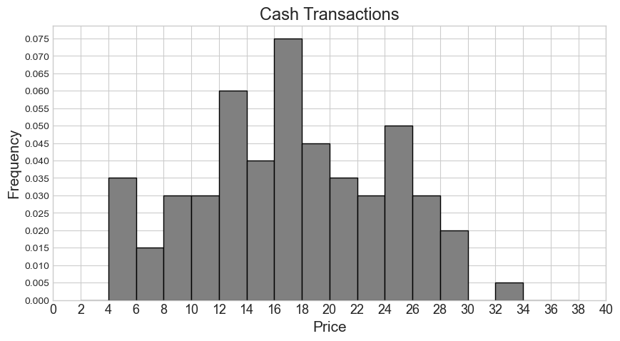
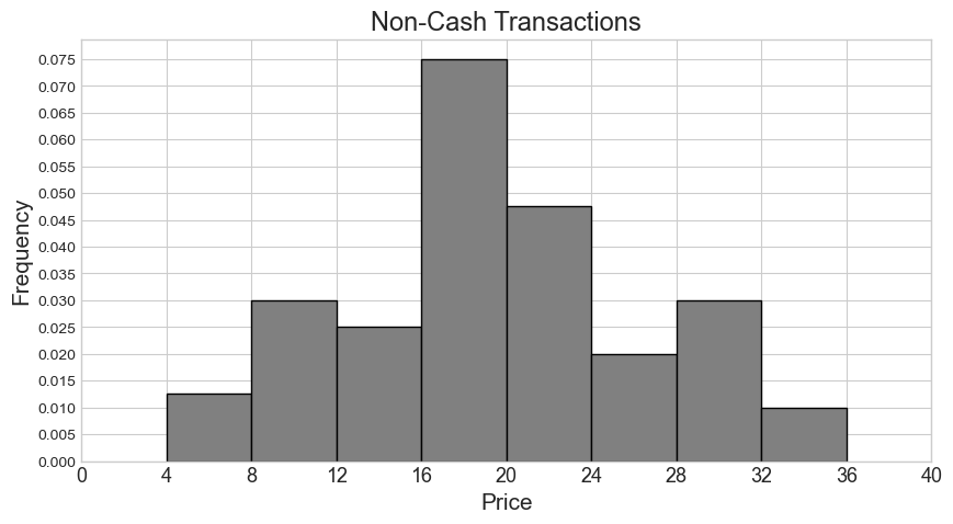
From these two histograms, we’d like to create a single combined
histogram that shows the overall distribution of "price"
for all 1000 rows in sales.
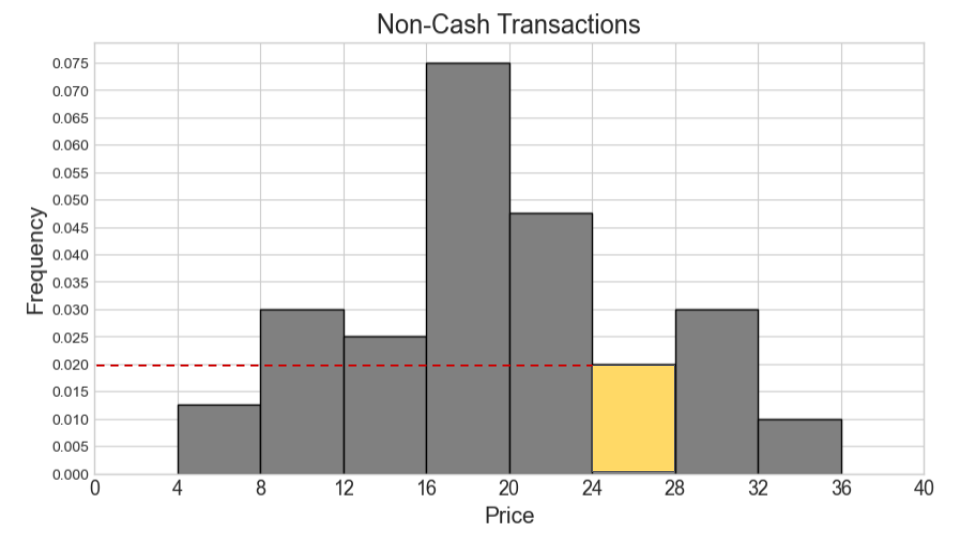
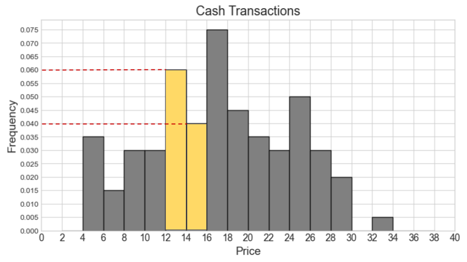
How many cash transactions had a "price" of \$26 or more?
Answer: 55
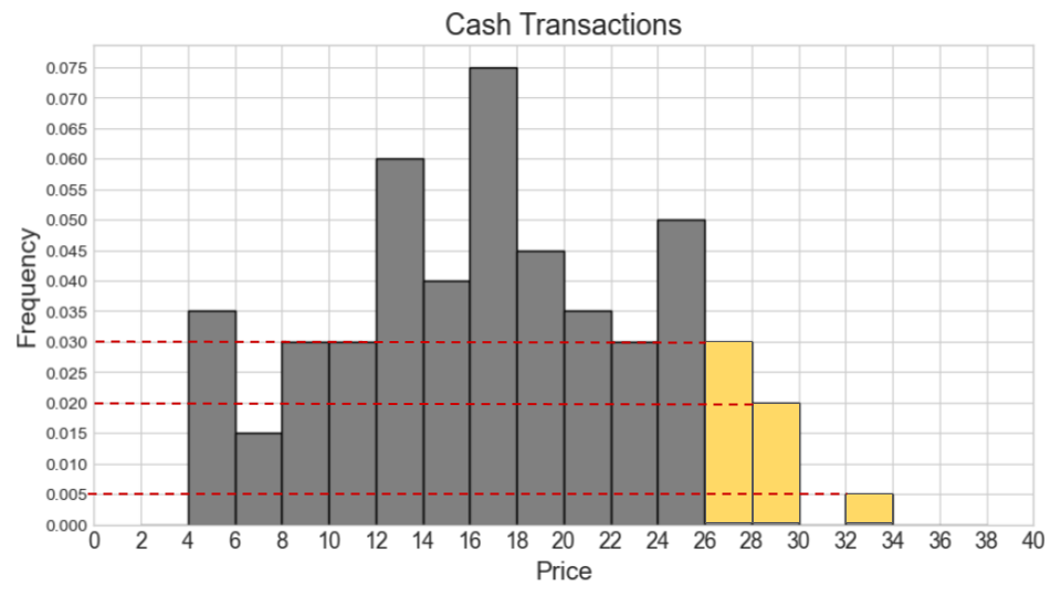
We first locate the bars representing \$26 or more on the cash transaction histogram, which are the three rightmost bars. We then calculate the area of these bars to get the proportion of cash transactions these bars correspond to.
\textit{Area} = 0.03 * 2 + 0.02 * 2 + 0.005 * 2 = 0.06 + 0.04 + 0.01 = 0.11
Lastly, we multiply this proportion by the total count of 500 to get
the count of transactions with a "price" of \$26 or more.
\text{number of transactions} = 0.11 * 500 = 55
The average score on this problem was 64%.
Say our combined histogram has a bin [4, 6). What will the height of this bar be in the combined histogram? Fill in the answer box or select “Not enough information.”
Answer: Not enough information.
Since the histogram for non-cash transactions only has a bin of [4, 8), we don’t have enough information about how many of these transactions fall within [4, 6). In general, we can’t tell where within a bin values fall in a histogram.
The average score on this problem was 81%.
Say our combined histogram has a bin [24, 28). What will the height of this bar be in the combined histogram? Fill in the answer box or select “Not enough information.”
Answer: 0.03
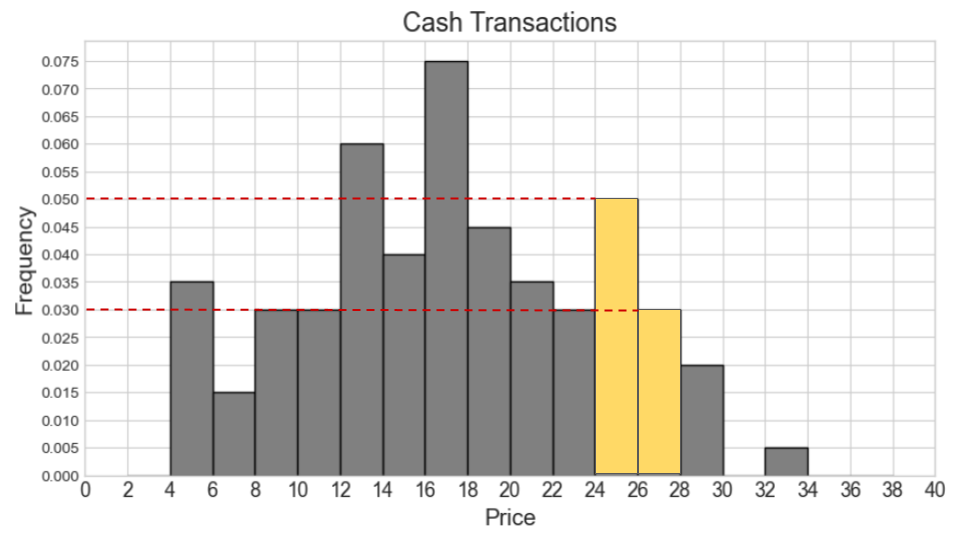
We first calculate the counts for cash and non-cash transactions within [24, 28) separately. Then we add the two counts and find the proportion this represents out of 1000 total transactions. Lastly, we determine the height of the bar by dividing the area (proportion) by the width 4.
Number of cash transactions within [24, 28) = (0.05 * 2 + 0.03 * 2) * 500 = (0.1 + 0.06) * 500 = 0.16 * 500 = 80
Number of non-cash transactions within [24, 28) = (0.02 * 4) * 500 = 0.08 * 500 = 40
Total number of transactions within [24, 28) = 80 + 40 = 120
Proportion of one thousand total transactions (area of bar) = 120 / 1000 = 0.12
Height of bar = 0.12 / 4 = 0.03
The average score on this problem was 42%.
Suppose now that the histograms for cash and non-cash transactions are the same as pictured, but they now represent 600 cash transactions and 400 non-cash transactions. In this situation, say our combined histogram has a bin [12, 16). What will the height of this bar be in the combined histogram? Fill in the answer box or select “Not enough information.”
Answer: 0.04
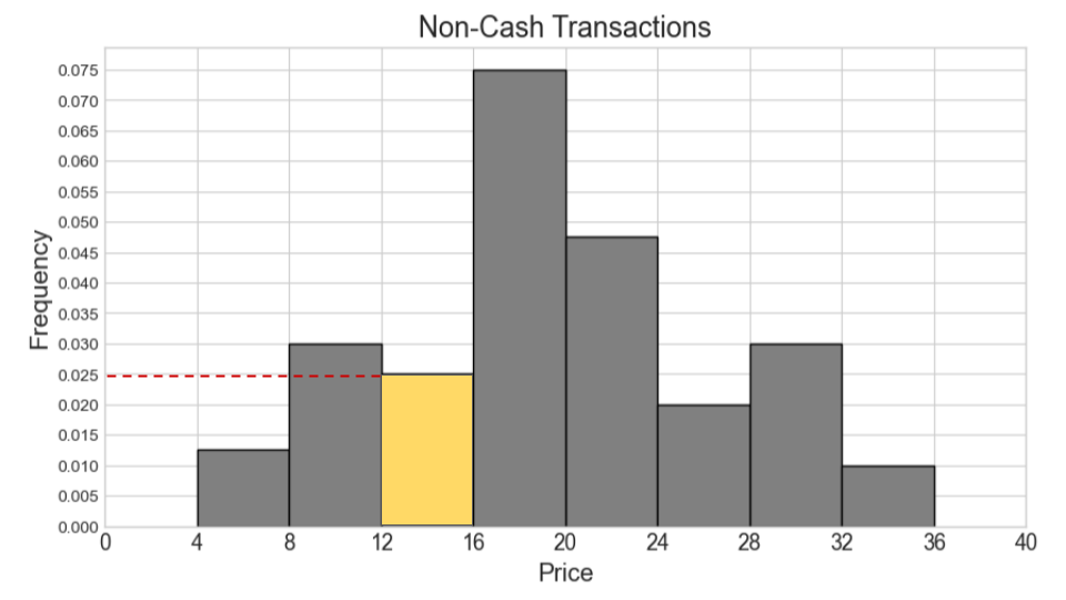
We can use the same process as we used for the previous part. We first calculate the counts for cash and non-cash transactions within [12, 16) separately. Then we add the two counts and find the proportion this represents out of 1000 total transactions. Lastly, we determine the height of the bar by dividing the area (proportion) by the width 4.
Number of cash transactions within [12, 16) = (0.06 * 2 + 0.04 * 2) * 600 = (0.12 + 0.08) * 600 = 0.2 * 600 = 120
Number of non-cash transactions within [12, 16) = (0.025 * 4) * 400 = 0.1 * 400 = 40
Total number of transactions within [12, 16) = 120 + 40 = 160
Proportion of one thousand total transactions (area of bar) = 160 / 1000 = 0.16
Height of bar = 0.16 / 4 = 0.04
The average score on this problem was 37%.
As in the previous problem, suppose we are told that
sales contains 1000 rows, 500 of which represent cash
transactions and 500 of which represent non-cash transactions.
This time, instead of being given histograms, we are told that the
distribution of "price" for cash transactions is roughly
normal, with a mean of \$14 and a
standard deviation of \$2. We’ll call
this distribution the cash curve.
Additionally, the distribution of "price" for non-cash
transactions is roughly normal, with a mean of \$22 and a standard deviation of \$4. We’ll call this distribution the
non-cash curve.
We want to draw a curve representing the approximate distribution of
"price" for all transactions combined. We’ll call this
distribution the combined curve.
What is the approximate proportion of area under the cash curve between \$10 and \$12? Your answer should be a number between 0 and 1.
Answer: 0.135
We know that for a normal distribution, approximately
For the cash curve, the mean is $14 and the standard deviation is $2, so using this rule:
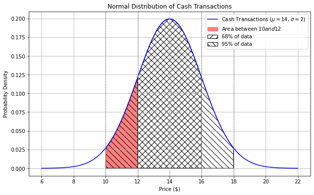
Area from $10 to $12 = Area from $10 to $14 - Area from $12 to $14 = 47.5% - 34% = 13.5% = 0.135
The average score on this problem was 46%.
Fill in the blanks in the code below so that the expression evaluates to the approximate proportion of area under the cash curve between \$14.50 and \$17.50. Each answer should be a single number.
scipy.stats.norm.cdf(a) - scipy.stats.norm.cdf(b)(a). Answer: 1.75
(b). Answer: 0.25
The expression
scipy.stats.norm.cdf(a) - scipy.stats.norm.cdf(b)
calculates the area under the normal distribution curve between two
points, where a is the right endpoint and b is
the left endpoint. Here, we’ll let a and b
represent the standardized values corresponding to $17.50 and $14.50,
respectively.
We’ll use the formula for standard units:
x_{i \: \text{(su)}} = \frac{x_i - \text{mean of $x$}}{\text{SD of $x$}}
For the standard units value corresponding to $17.50:
a = \frac{(17.50 - 14)}{2} = 1.75
For the standard units value corresponding to $14.50:
b = \frac{(14.50 - 14)}{2} = 0.25
The average score on this problem was 54%.
Will the combined curve be roughly normal?
Yes, because of the Central Limit Theorem.
Yes, because combining two normal distributions always produces a normal distribution.
No, not necessarily.
Answer: No, not necessarily.
Although both distributions are roughly normal, their means are significantly apart - one centered at 14 (with a standard deviation of 2) and one centered at 22 (with a standard deviation of 4). The resulting distribution is likely bimodal (having two peaks). The combined distribution will have peaks near each of the original means, reflecting the characteristics of the two separate normal distributions.
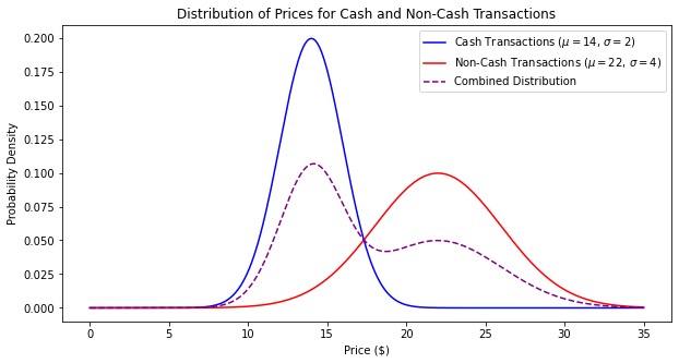
The CLT says that “the distribution of possible sample means is approximately normal, no matter the distribution of the population,” but it doesn’t say anything about combining two distributions.
The average score on this problem was 38%.
Fill in the blanks in the code below so that the expression evaluates to the approximate proportion of area under the combined curve between \$14 and \$22. Each answer should be a single number.
(scipy.stats.norm.cdf(a) - scipy.stats.norm.cdf(b)) / 2(a). Answer: 4
(b). Answer: -2
Since the the combined curve is a combination of two normal distributions, each representing equal number of transactions (500 each), we can approximate the total area by averaging the areas under the individual cash and non-cash curves between \$14 and \$22.
For cash:
P(Z ≤ \frac{22-14}{2}) - P(Z ≤ \frac{14-14}{2})
P(Z ≤ 4) - P(Z ≤ 0) = scipy.stats.norm.cdf(4) - scipy.stats.norm.cdf(0)
Non-cash:
P(Z ≤ \frac{22-22}{4}) - P(Z ≤ \frac{14-22}{4})
P(Z ≤ 0) - P(Z ≤ -2) = scipy.stats.norm.cdf(0) - scipy.stats.norm.cdf(-2)
Averaging area under the two distributions:
\frac{1}{2} (scipy.stats.norm.cdf(4) - scipy.stats.norm.cdf(0) + scipy.stats.norm.cdf(0) - scipy.stats.norm.cdf(-2)) = (scipy.stats.norm.cdf(4) - scipy.stats.norm.cdf(-2)) / 2
The average score on this problem was 15%.
What is the approximate proportion of area under the combined curve between \$14 and \$22? Choose the closest answer below.
0.47
0.49
0.5
0.95
0.97
Answer: 0.49
We can approximate the total area by averaging the areas under the individual cash and non-cash curves between \$14 and \$22.
Averaging the two individual areas: \frac{0.5 + 0.475}{2} = 0.4875, which is closest to 0.49.
The average score on this problem was 24%.
Suppose the bookstore DataFrame has 10 unique genres, and we are given a sample
of 350 books from that DataFrame.
Determine the maximum possible total variation distance (TVD) that could
occur between our sample’s genre distribution and the uniform
distribution where each genre occurs with equal probability. Your answer
should be a single number.
Answer: 0.9
To determine the maximum possible TVD, we consider the scenario where all books belong to a single genre. This represents the maximum deviation from the uniform distribution:
TVD = \frac{1}{2} \left( |1 - 0.1| + 9 \times |0 - 0.1| \right) = \frac{1}{2} (0.9 + 0.9) = 0.9
The average score on this problem was 31%.
True or False: If the sample instead had 700 books, then the maximum possible TVD would increase.
True
False
Answer: False
The maximum possible TVD is based on proportions and not absolute counts. Even if the sample size is increased, the TVD would remain the same.
The average score on this problem was 71%.
True or False: If the bookstore DataFrame had 11 genres
instead of 10, the maximum possible TVD would
increase.
True
False
Answer: True
With 11 genres, the uniform probability per genre decreases to \frac{1}{11} instead of \frac{1}{10} with 10 genres. In the extreme scenario where one genre dominates, the TVD is now bigger.
TVD = \frac{1}{2} \left( |1 - \frac{1}{11}| + 10 \times |0 - \frac{1}{11}| \right) = \frac{1}{2} (\frac{10}{11} + \frac{10}{11}) = \frac{10}{11}
The average score on this problem was 66%.
Dhruv works at the bookstore, and his job involves pricing new books that come in from the supplier. He prices new books based on the number of pages they have. He does this using linear regression, which he learned about in DSC 10.
To build his regression line, Dhruv gathers the following information about the distinct books currently available at the bookstore:
The correlation between price and number of pages is 0.6.
The mean price of all books is $15, with a standard deviation of $4.
The mean number of pages of all books is 500, with a standard deviation of 200.
Which of the following statements about Dhruv’s regression line are true? Select all that apply.
It goes through the point (500, 15).
It goes through the point (200, 4).
Its slope is equal to 0.6.
Its y-intercept is equal to 9.
Its root mean square error is larger than the root mean square error of any other line.
All the books currently available at the bookstore fall on the line.
Answer: a, d
When performing linear regression analysis, the slope
(m) and intercept (b) of the regression line
can be calculated as follows:
m = r \cdot \frac{\text{SD of } y}{\text{SD of } x} = 0.6 \times \left(\frac{4}{200}\right) = 0.012
b = (\text{mean of } y) - m \cdot (\text{mean of } x) = 15 - 0.012 \times 500 = 9
To predict the dependent variable (y_i) based on the independent variable (x_i): \text{predicted } y_i = 0.012 \cdot x_i + 9
True. The regression line will always pass through the point (\bar{x}, \bar{y}) due to the way we calculate it, which is (500, 15) in this case.
False. y = 0.012 \cdot 200 + 9 = 2.4 + 9 = 11.4 \neq 4
False. As calculated, the slope of the regression line is 0.012, not 0.6. The correlation coefficient is not the slope.
True. The intercept, based on the mean values and the calculated slope, is 9.
False. The least squares regression line minimizes the root mean square error (RMSE) compared to any other possible regression lines.
False. Regression provides a prediction or estimation, not an exact accounting. Not all books will fall exactly on the regression line due to the inherent variability and other influencing factors not accounted for in the simple linear model.
The average score on this problem was 80%.
If "The Martian" has 30
more pages than "The Simple Wild", and both books are
priced according to the regression line, how much more does
"The Martian" cost than "The Simple Wild"?
Give your answer as a number, in dollars and cents.
Answer: 0.36
Given the regression equation(calculated in previous question): \text{predicted } y_i = 0.012 \cdot x_i + 9
Assume:
x_i for “The Simple Wild” is x.
x_j for “The Martian” is x + 30.
Predicted price for “The Simple Wild” (y_i): y_i = 0.012 \cdot x + 9
Predicted price for “The Martian” (y_j): y_j = 0.012 \cdot (x + 30) + 9 y_j = 0.012 \cdot x + 0.36 + 9 y_j = 0.012 \cdot x + 9.36
The price of “The Martian” minus the price of “The Simple Wild”: y_j - y_i = (0.012 \cdot x + 9.36) - (0.012 \cdot x + 9) = 9.36 - 9 = 0.36
The average score on this problem was 39%.
A new book added to the inventory is "The Goldfinch",
which has 700 pages. How much should
Dhruv charge customers for this book, according to the regression line
pricing model? Give your answer as a number, in dollars and cents.
Answer: 17.4
Given the regression equation(calculated in (a)): \text{predicted } y_i = 0.012 \cdot x_i + 9
“The Goldfinch” has 700 pages. Substitute into the regression equation: y_i = 0.012 \cdot 700 + 9 = 8.4 + 9 = 17.4
The average score on this problem was 51%.
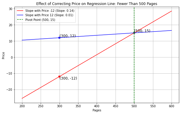
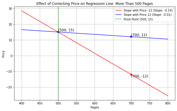
It turns out that Dhruv had an error in his regression line because
he had accidentally recorded the price of one book in the data set,
"Roadside Picnic", as -\$12 instead of \$12. He builds a new regression line using
the correct price for "Roadside Picnic" and he finds that
his new regression line has a smaller slope than before. What can we
conclude about the number of pages in "Roadside Picnic"
based on this information alone?
"Roadside Picnic" has fewer than 500 pages.
"Roadside Picnic" has exactly 500 pages.
"Roadside Picnic" has more than 500 pages.
Not enough information.
Answer: "Roadside Picnic" has fewer
than 500 pages.
The linear regression line has to pass through the point (500, 15).
Fewer Than 500 Pages: If “Roadside Picnic” has fewer than 500
pages, then this point is toward the left side of the pivot point of the
regression line, and price -12 will drag the line down(towards the lower
left corner) more than 12 does, so the slope will decrease if price
changes from -12 to 12.
Plot for your reference:
Exactly 500 Pages: If the book has exactly 500 pages, which is the mean or center of the data distribution, the incorrect price would mainly influence the intercept rather than the slope. Correcting the price would adjust the intercept but have a lesser effect on the slope.
More Than 500 Pages: If “Roadside Picnic” has more than 500
pages, then it’s toward the right side of the regression line, and price
-12 will drag the line down(towards the lower right corner) more than 12
does, so correcting this error would increase the slope.
Plot for your reference:
The average score on this problem was 49%.
Suppose that Dhruv originally based his regression line on a data set which has a single row for each unique book sold at Bill’s Book Bonanza. If instead, he had used a dataset with one row for each copy of a book at the bookstore (and there are multiple copies of some books), would his regression line have come out the same?
Yes
No
Answer: No
The regression line would not be the same due to the change in data and the resulting impact on mean and standard deviation of the price and pages.
The average score on this problem was 65%.
Suppose Dhruv bootstraps his scatterplot 10,000 times and calculates a regression line for each resample. It turns out that 95\% of his bootstrapped slopes fall in the interval [a, b] and 95\% of his bootstrapped intercepts fall in the interval [c, d]. Does this mean that 95\% of his predicted prices for a book with 500 pages fall in the interval [500a+c, 500b+d]?
Yes
No
Answer: No
95% of bootstrapped slopes and intercepts fall within specific intervals does not imply that 95% of predicted prices for a book with 500 pages will also fall within the interval [500a + c, 500b + d]. Because the intervals for slopes and intercepts are calculated independently, their combination does not account for the covariance between these regression parameters or the error variance around predictions. Additionally, combining slope and intercept independently can result in regression lines that do not pass through the pivotal point (mean(X), mean(Y)), making them unreliable for accurate prediction.
The average score on this problem was 55%.