← return to practice.dsc10.com
Below are practice problems tagged for Lecture 13 (rendered directly from the original exam/quiz sources).
Which of the following blocks of code correctly assigns
random_art_museums to an array of the names of 10 art
museums, randomly selected without replacement from those in
art_museums? Select all that apply.
Option 1:
def get_10(df):
    return np.array(df.sample(10).get('Name'))

random_art_museums = get_10(art_museums)
Option 2:
def get_10(art_museums):
    return np.array(art_museums.sample(10).get('Name'))

random_art_museums = get_10(art_museums)
Option 3:
def get_10(art_museums):
    random_art_museums = np.array(art_museums.sample(10).get('Name'))

random_art_museums = get_10(art_museums)
Option 4:
def get_10():
    return np.array(art_museums.sample(10).get('Name'))

random_art_museums = get_10()
Option 5:
random_art_museums = np.array([])

def get_10():
    random_art_museums = np.array(art_museums.sample(10).get('Name'))
    return random_art_museums

get_10()
Option 1
Option 2
Option 3
Option 4
Option 5
None of the above
Answers: Option 1, Option 2, and Option 4
Note that if df is a DataFrame, then
df.sample(10) is a DataFrame containing 10 randomly
selected rows in df. With that in mind, let’s look at all
of our options.
get_10 takes in a DataFrame df and returns an
array containing 10 randomly selected values in df’s
'Name' column. After defining get_10, we
assign random_art_museums to the result of calling
get_10(art_museums). This assigns
random_art_museums as intended, so Option 1 is
correct.art_museums and Option 1 uses the parameter name
df (both in the def line and in the function
body); this does not change the behavior of get_10 or the
lines afterward.get_10 here does not return
anything! So, get_10(art_museums) evaluates to
None (which means “nothing” in Python), and
random_art_museums is also None, meaning
Option 3 is incorrect.get_10 does not take in any inputs. However,
the body of get_10 contains a reference to the DataFrame
art_museums, which is ultimately where we want to sample
from. As a result, get_10 does indeed return an array
containing 10 randomly selected museum names, and
random_art_museums = get_10() correctly assigns
random_art_museums to this array, so Option 4 is
correct.get_10 returns the
correct array. However, outside of the function,
random_art_museums is never assigned to the output of
get_10. (The variable name random_art_museums
inside the function has nothing to do with the array defined before and
outside the function.) As a result, after running the line
get_10() at the bottom of the code block,
random_art_museums is still an empty array, and as such,
Option 5 is incorrect.
The average score on this problem was 85%.
London has the most art museums in the top 100 of any city in the
world. The most visited art museum in London is
'Tate Modern'.
Which of the following blocks of code correctly assigns
best_in_london to 'Tate Modern'? Select all
that apply.
Option 1:
def most_common(df, col):
    return df.groupby(col).count().sort_values(by='Rank', ascending=False).index[0]

def most_visited(df, col, value):
    return df[df.get(col)==value].sort_values(by='Visitors', ascending=False).get('Name').iloc[0]

best_in_london = most_visited(art_museums, 'City', most_common(art_museums, 'City'))
Option 2:
def most_common(df, col):
    print(df.groupby(col).count().sort_values(by='Rank', ascending=False).index[0])

def most_visited(df, col, value):
    print(df[df.get(col)==value].sort_values(by='Visitors', ascending=False).get('Name').iloc[0])

best_in_london = most_visited(art_museums, 'City', most_common(art_museums, 'City'))
Option 3:
def most_common(df, col):
    return df.groupby(col).count().sort_values(by='Rank', ascending=False).index[0]

def most_visited(df, col, value):
    print(df[df.get(col)==value].sort_values(by='Visitors', ascending=False).get('Name').iloc[0])

best_in_london = most_visited(art_museums, 'City', most_common(art_museums, 'City'))
Option 1
Option 2
Option 3
None of the above
Answer: Option 1 only
At a glance, it may seem like there’s a lot of reading to do to
answer the question. However, it turns out that all 3 options follow
similar logic; the difference is in their use of print and
return statements. Whenever we want to “save” the output of
a function to a variable name or use it in another function, we need to
return somewhere within our function. Only Option 1
contains a return statement in both
most_common and most_visited, so it is the
only correct option.
Let’s walk through the logic of Option 1 (which we don’t necessarily need to do to answer the problem, but we should in order to enhance our understanding):
most_common to find the city with the
most art museums. most_common does this by grouping the
input DataFrame df (art_museums, in this case)
by 'City' and using the .count() method to
find the number of rows per 'City'. Note that when using
.count(), all columns in the aggregated DataFrame will
contain the same information, so it doesn’t matter which column you use
to extract the counts per group. After sorting by one of these columns
('Rank', in this case) in decreasing order,
most_common takes the first value in the
index, which will be the name of the 'City'
with the most art museums. This is London,
i.e. most_common(art_museums, 'City') evaluates to
'London' in Option 1 (in Option 2, it evaluates to
None, since most_common there doesn’t
return anything).most_visited to find the museum with the
most visitors in the city with the most museums. This is achieved by
keeping only the rows of the input DataFrame df (again,
art_museums in this case) where the value in the
col ('City') column is value
(most_common(art_museums, 'City'), or
'London'). Now that we only have information for museums in
London, we can sort by 'Visitors' to find the most visited
such museum, and take the first value from the resulting
'Name' column. While all 3 options follow this logic, only
Option 1 returns the desired value, and so only Option
1 assigns best_in_london correctly. (Even if Option 2’s
most_visited used return instead of
print, it still wouldn’t work, since Option 2’s
most_common also uses print instead of
return).
The average score on this problem was 86%.
Since txn has 140,000 rows, Jack wants to get a quick
glimpse at the data by looking at a simple random sample of 10 rows from
txn. He defines the DataFrame ten_txns as
follows:
ten_txns = txn.sample(10, replace=False)Which of the following code blocks also assign ten_txns
to a simple random sample of 10 rows from txn?
Option 1:
    all_rows = np.arange(txn.shape[0])
    perm = np.random.permutation(all_rows)
    positions = np.random.choice(perm, size=10, replace=False)
    ten_txn = txn.take(positions)
Option 2:
    all_rows = np.arange(txn.shape[0])
    choice = np.random.choice(all_rows, size=10, replace=False)
    positions = np.random.permutation(choice)
    ten_txn = txn.take(positions)
Option 3:
    all_rows = np.arange(txn.shape[0])
    positions = np.random.permutation(all_rows).take(np.arange(10))
    ten_txn = txn.take(positions)
Option 4:
    all_rows = np.arange(txn.shape[0])
    positions = np.random.permutation(all_rows.take(np.arange(10)))
    ten_txn = txn.take(positions)
Select all that apply.
Option 1
Option 2
Option 3
Option 4
None of the above.
Answer: Option 1, Option 2, and Option 3.
Let’s consider each option.
Option 1: First, all_rows is defined as an array
containing the integer positions of all the rows in the DataFrame. Then,
we randomly shuffle the elements in this array and store it in the array
permutations. Finally, we select 10 integers randomly
(without replacement), and use .take() to select the rows
from the DataFrame with the corresponding integer locations. In other
words, we are randomly selecting ten row numbers and taking those
randomly selected. This gives a simple random sample of 10 rows from the
DataFrame txn, so option 1 is correct.
Option 2: Option 2 is similar to option 1, except that the order
of the np.random.choice and the
np.random.permutation operations are switched. This doesn’t
affect the output, since the choice we made was, by definition, random.
Therefore, it doesn’t matter if we shuffle the rows before or after (or
not at all), since the most this will do is change the order of a sample
which was already randomly selected. So, option 2 is correct.
Option 3: Here, we randomly shuffle the elements of
all_rows, and then we select the first 10 elements with
np.take. Since the shuffling of elements from
all_rows was random, we don’t know which elements are in
the first 10 positions of this new shuffled array (in other words, the
first 10 elements are random). So, when we select the rows from
txn which have the corresponding integer locations in the
next step, we’ve simply selected 10 rows with random integer locations.
Therefore, this is a valid random sample from txn, and
option 3 is correct.
Option 4: The difference between this option and option 3 is the
order in which np.random.permutation and
np.take are executed. Here, we select the first 10 elements
before the permutation (inside the parentheses). As a result, the array
which we’re shuffling with np.random.permutation does not
include all the integer locations like all_rows does, it’s
simply the first ten elements. Therefore, this code produces a random
shuffling of the first 10 rows of txn, which is not a
random sample.
The average score on this problem was 82%.
We want to use app_data to estimate the average amount
of time it takes to build an IKEA bed (any product in the
'bed' category). Which of the following strategies would be
an appropriate way to estimate this quantity? Select all that apply.
Query to keep only the beds. Then resample with replacement many
times. For each resample, take the mean of the 'minutes'
column. Compute a 95% confidence interval based on those means.
Query to keep only the beds. Group by 'product' using
the mean aggregation function. Then resample with replacement many
times. For each resample, take the mean of the 'minutes'
column. Compute a 95% confidence interval based on those means.
Resample with replacement many times. For each resample, first query
to keep only the beds and then take the mean of the
'minutes' column. Compute a 95% confidence interval based
on those means.
Resample with replacement many times. For each resample, first query
to keep only the beds. Then group by 'product' using the
mean aggregation function, and finally take the mean of the
'minutes' column. Compute a 95% confidence interval based
on those means.
Answer: Option 1
Only the first answer is correct. This is a question of parameter estimation, so our approach is to use bootstrapping to create many resamples of our original sample, computing the average of each resample. Each resample should always be the same size as the original sample. The first answer choice accomplishes this by querying first to keep only the beds, then resampling from the DataFrame of beds only. This means resamples will have the same size as the original sample. Each resample’s mean will be computed, so we will have many resample means from which to construct our 95% confidence interval.
In the second answer choice, we are actually taking the mean twice.
We first average the build times for all builds of the same product when
grouping by product. This produces a DataFrame of different products
with the average build time for each. We then resample from this
DataFrame, computing the average of each resample. But this is a
resample of products, not of product builds. The size of the resample is
the number of unique products in app_data, not the number
of reported product builds in app_data. Further, we get
incorrect results by averaging numbers that are already averages. For
example, if 5 people build bed A and it takes them each 1 hour, and 1
person builds bed B and it takes them 10 hours, the average amount of
time to build a bed is \frac{5*1+10}{6} =
2.5. But if we average the times for bed A (1 hour) and average
the times for bed B (5 hours), then average those, we get \frac{1+5}{2} = 3, which is not the same.
More generally, grouping is not a part of the bootstrapping process
because we want each data value to be weighted equally.
The last two answer choices are incorrect because they involve
resampling from the full app_data DataFrame before querying
to keep only the beds. This is incorrect because it does not preserve
the sample size. For example, if app_data contains 1000
reported bed builds and 4000 other product builds, then the only
relevant data is the 1000 bed build times, so when we resample, we want
to consider another set of 1000 beds. If we resample from the full
app_data DataFrame, our resample will contain 5000 rows,
but the number of beds will be random, not necessarily 1000. If we query
first to keep only the beds, then resample, our resample will contain
exactly 1000 beds every time. As an added bonus, since we only care
about beds, it’s much faster to resample from a smaller DataFrame of
beds only than it is to resample from all app_data with
plenty of rows we don’t care about.
The average score on this problem was 71%.
Which of the following statements are true in general? Select all that apply.
Parameters are fixed, but statistics can change depending on the sample.
Parameters and statistics can both fluctuate depending on the sample.
For simple random samples, statistics give better estimates of parameters when the sample size is larger.
The distribution of a statistic is the same regardless of the sample size.
None of the above.
Options 1 and 3
The average score on this problem was 90%.
Which of the following can be used to generate a simple
random sample of "rating"s from 10 restaurants in
restaurants? Select all that apply.
Option 1:
sample = restaurants.take(np.arange(10)).get("rating")Option 2:
sample = restaurants.sample(10, replace = False).get("rating")Option 3:
sample = restaurants.sample(10, replace = True).get("rating")Option 4:
    positions = np.random.choice(np.arange(0, restaurants.shape[0]),
                                 10, replace = False)
    sample = restaurants.take(positions).get("rating")
Option 5:
    positions = np.random.choice(np.arange(0, restaurants.shape[0]),
                                 10, replace = True)
    sample = restaurants.take(positions).get("rating")
Option 1
Option 2
Option 3
Option 4
Option 5
Options 2 and 4
The average score on this problem was 65%.
Shivani wrote a function called doggos defined as
follows:
def doggos(n, lower, upper):
t = df.sample(n, replace=True).get('longevity')
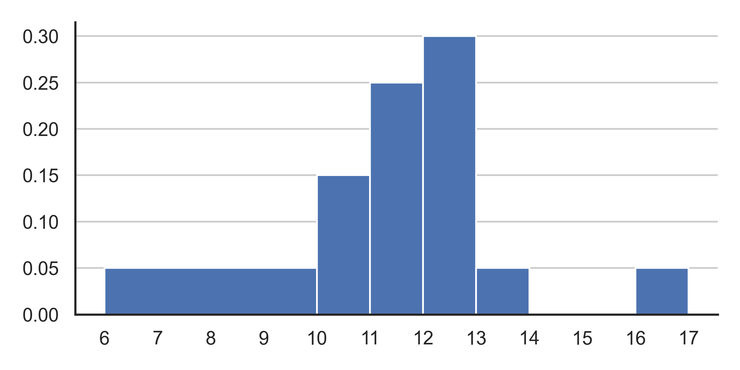
return sum(lower <= t < upper)This plot shows a density histogram of the 'longevity'
column.
Answer each of these questions by either writing a single number in the box or selecting “Not enough information”, but not both. What is the probability that:
doggos(1, 10, 11) == 1 is True?
Answer: 0.15
Let’s first understand the function. The function takes inputs
n, lower, and upper and randomly
takes a sample of n rows with replacement from DataFrame
df, gets column longevity from the sample and
saves it as a Series t. The n entries of
t are randomly generated according to the density histogram
shown in the picture. That is, the probability of a particular value
being generated in Series t for a given entry can be
visualized by the density histogram in the picture.
lower <= t < upper takes t and generates
a Series of boolean values, either True or
False depending on whether the corresponding entry in
t lies within the range. And so
sum(lower <= t < upper) returns the number of entries
in t that lies between the range values. (This is because
True has a value of 1 and False has a value of
0, so summing Booleans is a quick way to count how many
True there are.)
Now part a is just asking for the probability that we’ll draw a
longevity value (given that n is
1, so we only draw one longevity value)
between 10 and 11 given the density plot. Note that the probability of a
bar is given by the width of the bar multiplied by the height. Now
looking at the bar with bin of range 10 to 11, we can see that the
probability is just (11-10) * 0.15 = 1 * 0.15
= 0.15.
The average score on this problem was 86%.
doggos(2, 0, 12) == 2 is True?
Answer: 0.36
Part b is essentially asking us: What is the probability that after
drawing two longevity values according to the density plot,
both of them will lie in between 0 and 12?
Let’s first start by considering the probability of drawing 1
longevity value that lies between 0 and
12. This is simply just the sum of the areas of the three
bars of range 6-10, 10-11, and 11-12, which is just (4*0.05) + (1*0.15) + (1*0.25) = 0.6
Now because we draw each value independently from one another, we simply square this probability which gives us an answer of 0.6*0.6 = 0.36
The average score on this problem was 81%.
doggos(2, 13, 20) > 0 is True?
Answer: 0.19
Part c is essentially asking us: What is the probability that after
drawing two longevity values according to the density plot,
at least one of them will lie in between 12 and 20?
While you can directly solve for this probability, a faster method would be to solve for the complementary of this problem. That is, we can solve for the probability that none of them lie in between the given ranges. And once we solve this, we can simply subtract our answer from one, because the only options for this scenario is that either at least one of the values lie in between the range, or neither of the values do.
Again, let’s solve for the probability of drawing 1
longevity value that isn’t between the range. Staying true
to our complementary strategy, this is just 1 minus the probability of
drawing a longevity value that is in the
range, which is just 1 - (1*0.05+1*0.05) =
0.9
Again, because we draw each value independently, squaring this probability gives us the probability that neither of our drawn values are in the range, or 0.9*0.9 = 0.81. Finally, subtracting this from 1 gives us our desired answer or 1 - 0.81 =0.19
The average score on this problem was 66%.
You sample from a population by assigning each element of the
population a number starting with 1. You include element 1 in your
sample. Then you generate a random number, n, between 2 and
5, inclusive, and you take every nth element after element
1 to be in your sample. For example, if you select n=2,
then your sample will be elements 1, 3, 5, 7, and so
on.
True or False: Before the sample is drawn, you can calculate the probability of selecting each subset of the population.
Answer: True
The answer is true since someone can easily sketch each sample to view the probability of selecting a certain subset. For example, when n = 2 we know the elements are 1, 3, 5, 7, and so on. Similarly we know this information for n = 3, 4 and 5. Using this information we could calculate the probability of selecting a subset.
The average score on this problem was 97%.
True or False: Each subset of the population is equally likely to be selected.
Answer: False
No, each subset of the population is not equally likely to be selected since the element assigned as element 1 will always be selected due to the way sampling is conducted as defined in the question. That is, the question says we always include element one in the sample which will over represent it in samples as compared to other parts of the population.
The average score on this problem was 46%.
Assume df is a DataFrame with distinct rows. Which of
the following best describes df.sample(10)?
an array of length 10, where some of the entries might be the same
an array of length 10, where no two entries can be the same
a DataFrame with 10 rows, where some of the rows might be the same
a DataFrame with 10 rows, where no two rows can be the same
Answer: a DataFrame with 10 rows, where no two rows can be the same
Looking at the documentation for .sample() we can see
that it accepts a few arguments. The first argument specifies the number
of rows (which is why we specify 10). The next argument is a boolean
that specifies if the sampling happens with or without replacement. By
default, the sampling will occur without replacement (which happens in
this question since no argument is specified so the default is evoked).
Looking at the return, we can see that since we are sampling a
dataframe, a dataframe will also be returned which is why a DataFrame
with 10 rows, where no two rows can be the same is correct.
The average score on this problem was 94%.
Describe in your own words the difference between a probability distribution and an empirical distribution. Give an example of what each distribution might look like for a certain experiment. Choose an experiment that we have not already seen in this class.
Answer: There are many possible correct answers. Below are some student responses that earned full credit, lightly edited for clarity.
Probability distributions are theoretical distributions distributed over all possible values of an experiment. Meanwhile, empirical distributions are distributions of the real observed data. An example of this would be choosing a certain suit from a deck of cards. The probability distribution would be uniform, with a 1/4 chance of choosing each suit. Meanwhile, the empirical distribution of choosing suits from a deck of cards in 50 pulls manually and graphing the observed data would show us different chances.
A probability distribution is the distribution describing the theoretical probability of each potential value occurring in an experiment, while the empirical distribution describes the proportion of each of the values in the experiment after running it, including all observed values. In other words, the probability distribution is what we expect to happen, and the empirical distribution is what actually happens.
For example: My friends and I often go to a food court to eat, and we randomly pick a restaurant every time. There is 1 McDonald’s, 1 Subway, and 2 Panda Express restaurants in the food court.
The probability distribution is as follows:
After going to the food court 100 times, we look at the empirical distribution to see which restaurants we eat at most often. it is as follows:
Probability distribution is a theoretical representation of certain outcomes in an event whereas an empirical distribution is the observational representation of the same outcomes in an event produced from an experiment.
An example would be if I had 10 pairs of shoes in my closet: The probability distribution would suggest that each pair of shoes has an equal chance of getting picked on any given day. On the other hand, an empirical distribution would be drawn by recording which pair got picked on a given day in N trials.
The average score on this problem was 82%.
results = np.array([])
for i in np.arange(10):
    result = np.random.choice(np.arange(1000), replace=False)
    results = np.append(results, result)
After this code executes, results contains:
a simple random sample of size 9, chosen from a set of size 999 with replacement
a simple random sample of size 9, chosen from a set of size 999 without replacement
a simple random sample of size 10, chosen from a set of size 1000 with replacement
a simple random sample of size 10, chosen from a set of size 1000 without replacement
Answer: a simple random sample of size 10, chosen from a set of size 1000 with replacement
Let’s see what the code is doing. The first line initializes an empty
array called results. The for loop runs 10 times. Each
time, it creates a value called result by some process
we’ll inspect shortly and appends this value to the end of the
results array. At the end of the code snippet,
results will be an array containing 10 elements.
Now, let’s look at the process by which each element
result is generated. Each result is a random
element chosen from np.arange(1000) which is the numbers
from 0 to 999, inclusive. That’s 1000 possible numbers. Each time
np.random.choice is called, just one value is chosen from
this set of 1000 possible numbers.
When we sample just one element from a set of values, sampling with replacement is the same as sampling without replacement, because sampling with or without replacement concerns whether subsequent draws can be the same as previous ones. When we’re just sampling one element, it really doesn’t matter whether our process involves putting that element back, as we’re not going to draw again!
Therefore, result is just one random number chosen from
the 1000 possible numbers. Each time the for loop executes,
result gets set to a random number chosen from the 1000
possible numbers. It is possible (though unlikely) that the random
result of the first execution of the loop matches the
result of the second execution of the loop. More generally,
there can be repeated values in the results array since
each entry of this array is independently drawn from the same set of
possibilities. Since repetitions are possible, this means the sample is
drawn with replacement.
Therefore, the results array contains a sample of size
10 chosen from a set of size 1000 with replacement. This is called a
“simple random sample” because each possible sample of 10 values is
equally likely, which comes from the fact that
np.random.choice chooses each possible value with equal
probability by default.
The average score on this problem was 11%.
Suppose we take a uniform random sample with replacement from a population, and use the sample mean as an estimate for the population mean. Which of the following is correct?
If we take a larger sample, our sample mean will be closer to the population mean.
If we take a smaller sample, our sample mean will be closer to the population mean.
If we take a larger sample, our sample mean is more likely to be close to the population mean than if we take a smaller sample.
If we take a smaller sample, our sample mean is more likely to be close to the population mean than if we take a larger sample.
Answer: If we take a larger sample, our sample mean is more likely to be close to the population mean than if we take a smaller sample.
Larger samples tend to give better estimates of the population mean than smaller samples. That’s because large samples are more like the population than small samples. We can see this in the extreme. Imagine a sample of 1 element from a population. The sample might vary a lot, depending on the distribution of the population. On the other extreme, if we sample the whole population, our sample mean will be exactly the same as the population mean.
Notice that the correct answer choice uses the words “is more likely to be close to” as opposed to “will be closer to.” We’re talking about a general phenomenon here: larger samples tend to give better estimates of the population mean than smaller samples. We cannot say that if we take a larger sample our sample mean “will be closer to” the population mean, since it’s always possible to get lucky with a small sample and unlucky with a large sample. That is, one particular small sample may happen to have a mean very close to the population mean, and one particular large sample may happen to have a mean that’s not so close to the population mean. This can happen, it’s just not likely to.
The average score on this problem was 100%.
As in the previous question, let coop_sample be a sample
of 100 rows of games, all corresponding to cooperative games.
Define samp and resamp as follows.
samp = coop_sample.get("Complexity")
resamp = coop_sample.sample(100, replace=True).get("Complexity")Which of the following statements could evaluate to True? Select all that are possible.
len(samp.unique()) < len(resamp.unique())
len(samp.unique()) == len(resamp.unique())
len(samp.unique()) > len(resamp.unique())
Answer: Options 2 and 3
Option 2: This is correct because it is possible for
resamp to be shuffled in such a way that the number of
unique elements are not the same.
Option 3: This is correct because it is possible for
resamp to pull the same values more often making it less
unique than samp.
Option 1: The reason that this is incorrect is
because samp.unique() has the most possible unique elements
inside of it. When we shuffle it using
coop_sample.sample(100, replace = True) we could pull the
same value multiple times, making it less unique.
The average score on this problem was 91%.
Which of the following statements could evaluate to True? Select all that are possible.
np.count nonzero(samp == 1) < np.count nonzero(resamp == 1)
np.count nonzero(samp == 1) == np.count nonzero(resamp == 1)
np.count nonzero(samp == 1) > np.count nonzero(resamp == 1)
Answer: Options 1, 2, and 3
Option 1: It might be helpful to recall what exactly
the column “Complexity” holds. In this case it holds the
average complexity of the game on a scale of 1 to 5. The code is trying
to find if the number of ones in samp and
resamp are different. It is possible that when shuffling
due to replace = True that resamp has more
ones inside of it than samp.
Option 2: Once again it is possible that when
shuffled resamp has the same number of ones as
samp does.
Option 3: When we shuffle coop_sample
there is no guarantee that one will sample more ones and instead other
averages could be selected. This means it is possible for the number of
ones in samp can be greater than the number of ones in
resamp.
The average score on this problem was 83%.
Which of the following statements could evaluate to True? Select all that are possible.
samp.min() < resamp.min()
samp.min() == resamp.min()
samp.min() > resamp.min()
Answer: Options 1 and 2
Option 1: It is possible when shuffled that
samp’s original minimum is never sampled, making
resamp’s minimum to be greater than samp’s
min.
Option 2: If samp’s original min is
sampled then it will be the same minimum that appears inside of
resamp.
Option 3: It is impossible for resamp’s
minimum to be less than samp’s minimum. This is because all
of resamp’s values come from samp. That means
there cannot be a smaller value inside of resamp that never
appears in samp.
The average score on this problem was 83%.
Which of the following statements could evaluate to True? Select all that are possible.
np.std(samp) < np.std(resamp)
np.std(samp) == np.std(resamp)
np.std(samp) > np.std(resamp)
Answer: Options 1, 2, and 3
Option 1: np.std() gives us the
standard deviation of the array we give it. When we do
np.std(samp) we are finding the standard deviation of
“Complexity”. When we do np.std(resamp) we are
finding the standard deviation of “Complexity”, which may
grab values multiple times. Since we are grabbing values multiple times
it is possible to have a standard deviation become smaller if we
continuously grab smaller values.
Option 2: If the resamp gets us the
same values as samp we would end up with the same standard
deviation, which would make
np.std(samp) == np.std(resamp).
Option 3: Similar to Option 1, we may grab many values which are on the larger end, which could increase our standard deviation.
The average score on this problem was 79%.
Suppose the function simulate_lcr from the last question
has been correctly implemented, and we want to use it to see how many
turns a game of Left, Center, Right usually takes.
Note: You can answer this question even if you couldn’t answer the previous one.
Consider the code and histogram below.
turns = np.array([])
for i in np.arange(10000):
    turns = np.append(turns, simulate_lcr())
(bpd.DataFrame().assign(turns=turns).plot(kind="hist", density = True, ec="w", bins = np.arange(0, 66, 6)))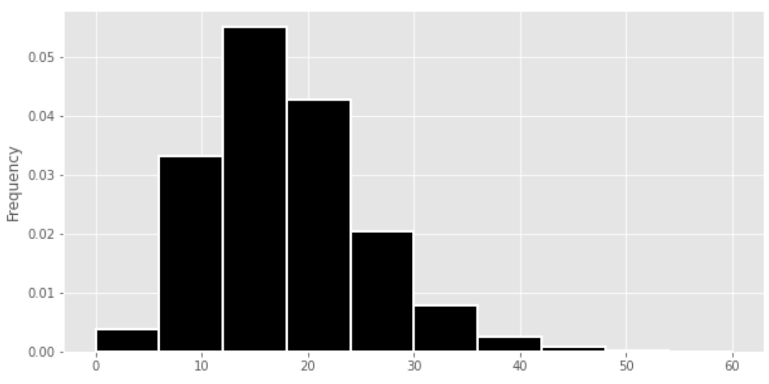
Does this histogram show a probability distribution or an empirical distribution?
Probability Distribution
Empirical Distribution
Answer: Empirical Distribution
An empirical distribution is derived from observed data, in this case, the results of 10,000 simulated games of Left, Center, Right. It represents the frequencies of outcomes (number of turns taken in each game) as observed in these simulations.
The average score on this problem was 54%.
What is the probability of a game of Left, Center, Right lasting 30 turns or more? Choose the closest answer below.
0.01
0.06
0.10
0.60
Answer: 0.06
We’re being asked to find the proportion of values in the histogram that are greater than or equal to 30, which is equal to the area of the histogram to the right of 30. Immediately, we can rule out 0.01 and 0.60, because the area to the right of 30 is more than 1% of the total area and less than 60% of the total area.
The problem then boils down to determining whether the area to the right of 30 is 0.06 or 0.10. While you could solve this by finding the areas of the three bars individually and adding them together, there’s a quicker solution. Notice that the x-axis gridlines – the vertical lines in the background in white – appear every 10 units (at x = 0, x = 10, x = 20, x = 30, and so on) and the y-axis gridlines – the horizontal lines in the background in white – appear every 0.01 units (at y = 0, y = 0.01, y = 0.02, and so on). There’s a “box” in the grid between x = 30 and x = 40, and between y = 0 and y = 0.01. The area of that box is (40 - 30) \cdot 0.01 = 0.1, which means that if a bar book up the entire box, then 10% of the values in this distribution would fall into that bar’s bin.
So, to decide whether the area to the right of 30 is closer to 0.06 or 0.1, we can estimate whether the three bars to the right of 30 would fill up the entire box described above (that is, the box from 30 to 40 on the x-axis and 0 to 0.1 on the y-axis), or whether it would be much emptier. Visually, if you broke off the area that is to the right of 40 in the histogram and put it in the box we’ve just described, then quite a bit of the box would still be empty. As such, the area to the right of 30 is less than the area of the box, so it’s less than 0.1, and so the only valid option is 0.06.
The average score on this problem was 50%.
Suppose a player with n chips takes their turn. What is the probability that they will have to put at least one chip into the center? Give your answer as a mathematical expression involving n.
Answer: 1 - (\frac{5}{6})^n
Recall that the die used to play this game has six sides: L, C, R, Dot, Dot, Dot. The chance of getting C is \frac{1}{6}. So we can take the complement of that to get \frac{5}{6}, which is the probability of not putting at least one chip into the center and then doing (\frac{5}{6})^n. Once again we must use the complement rule to convert it back to the probability of putting at least one chip into the center. This gives us the answer: 1 - (\frac{5}{6})^n
The average score on this problem was 56%.
Suppose a player with n chips takes their turn. What is the probability that they will end their turn with n chips? Give your answer as a mathematical expression involving n.
Answer: \left( \frac{1}{2} \right)^n
Recall, when it is a player’s turn, they roll one die for each of the n chips they have. The die that they roll has six faces. In three of those faces (L, C, and R), they end up losing a chip, and in the other three of those faces (dot, dot, and dot), they keep the chip. So, for each chip, there is a \frac{3}{6} = \frac{1}{2} chance that they get to keep it after the turn. Since each die roll is independent, there is a \frac{1}{2} \cdot \frac{1}{2} \cdot ... \cdot \frac{1}{2} = \left( \frac{1}{2} \right)^n chance that they get to keep all n chips. (Note that there is no way to earn more chips during a turn, so that’s not something we need to consider.)
The average score on this problem was 69%.
Select all sampling methods below where the
resulting sample is an SRS of 20 songs from the songs
DataFrame.
Use songs.sample(20, replace=1)
Use
np.random.multinomial(20, np.ones(songs.shape[0]) / songs.shape[0])
to decide how many times to take each row for a sample.
np.random.choice(songs.get("song_name"), 20)
Randomly pick 20 genres without replacement, then within each picked genre, randomly pick a song.
Randomly pick 20 artists without replacement, then within each picked artist, randomly pick a song.
None of the above.
Answer: None of the above
replace=1 means sampling
with replacement, which is not an SRS (SRS requires sampling without
replacement).np.random.multinomial
assigns counts to rows and can select rows multiple times — this is
sampling with replacement, not SRS.np.random.choice on a column
samples values with replacement by default and doesn’t return full
rows.
The average score on this problem was 62%.