← return to practice.dsc10.com
Below are practice problems tagged for Lecture 15 (rendered directly from the original exam/quiz sources).
Suppose we have access to a simple random sample of all US Costco
members of size 145. Our sample is stored in a
DataFrame named us_sample, in which the
"Spend" column contains the October 2023 spending of each
sampled member in dollars.
Fill in the blanks:
"Spend" column in us_sample is a ____,
while the average October 2023 spending of all US members is a ____."
sample statistic; population parameter
population statistic; sample parameter
sample parameter; population statistic
population parameter; sample statistic
Answer: sample statistic; population parameter
The average score on this problem was 94%.
Fill in the blanks below so that us_left and
us_right are the left and right endpoints of a
46% confidence interval for the average October 2023
spending of all US members.
costco_means = np.array([])
for i in np.arange(5000):
    resampled_spends = __(x)__
    costco_means = np.append(costco_means, resampled_spends.mean())
left = np.percentile(costco_means, __(y)__)
right = np.percentile(costco_means, __(z)__)
Which of the following could go in blank (x)? Select all that apply.
us_sample.sample(145, replace=True).get("Spend")
us_sample.sample(145, replace=False).get("Spend")
np.random.choice(us_sample.get("Spend"), 145)
np.random.choice(us_sample.get("Spend"), 145, replace=True)
np.random.choice(us_sample.get("Spend"), 145, replace=False)
None of the above.
What goes in blanks (y) and (z)? Give your answers as integers.
Answer:
x:
us_sample.sample(145, replace=True).get("Spend")np.random.choice(us_sample.get("Spend"), 145)np.random.choice(us_sample.get("Spend"), 145, replace=True)y: 27z: 73
The average score on this problem was 79%.
True or False: 46% of all US members in
us_sample spent between left and
right in October 2023.
True
False
Answer: False
The average score on this problem was 85%.
True or False: If we repeat the code from part (b) 200 times, each time bootstrapping from a new random sample of 145 members drawn from all US members, then about 92 of the intervals we create will contain the average October 2023 spending of all US members.
True
False
Answer: True
The average score on this problem was 51%.
True or False: If we repeat the code from part (b) 200 times, each
time bootstrapping from us_sample, then about
92 of the intervals we create will contain the average
October 2023 spending of all US members.
True
False
Answer: False
The average score on this problem was 30%.
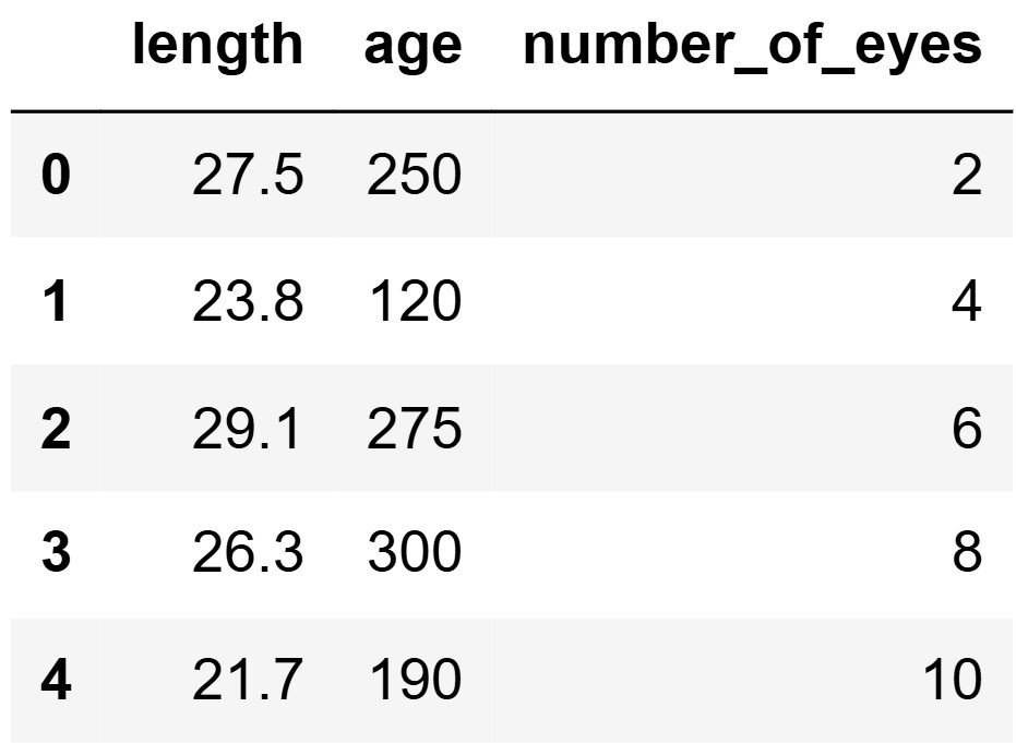
The DataFrame space_reptiles contains 1000 rows of
information about all space reptiles living on
Statistica, which we’ll think of as a population. For each reptile, we
have its "length" in meters, "age" in years,
and "number_of_eyes". The first five rows of
space_reptiles are shown below.
Fill in the blanks in the sample_of_reptiles function.
The function has two parameters, "sample_size" (int), which
will be a positive integer, and "column" (str), which will
be the name of one of the columns in space_reptiles. The
function should take a sample of reptiles from
space_reptiles, with replacement, of the
specified size, and return the average value in the given column for the
sample.
def sample_of_reptiles(sample_size, column):
return space_reptiles.sample(__(x)__).__(y)__ Answer:
x: sample_size, replace=True
y: get(column).mean()
The average score on this problem was 85%.
True or False: The function call
sample_of_reptiles(1000, "length") is an example of
bootstrapping.
Answer: False
The average score on this problem was 77%.
Calculate the variance of the data in the first five
rows of the "number_of_eyes" column of
space_reptiles: 2, 4, 6, 8, 10. Give your answer as an
integer.
Answer: 8
The average score on this problem was 50%.
Suppose the next row in the "number_of_eyes" column
contains 6. If we add this value to our dataset and then recompute the
variance, it would...
decrease because the new value is less than the greatest value
decrease because the new value is equal to the mean.
remain the same because the new value is equal to the median.
increase because the data set has more values than it did
increase because the new value is a positive number.
Answer: decrease because the new value is equal to the mean.
The average score on this problem was 62%.
A sleepy cat is a cat that naps for at least 5 hours. You want to
estimate the proportion of all sleepy cats that
consumed at least 10 treats, based on the data in cats.
Fill in the blanks below to generate an array of 10000 bootstrapped estimates for this proportion.
estimates = np.array([])
subset = cats[__(a)__]
for i in np.arange(10000):
    resample = __(b)__
    proportion = __(c)__ / __(d)__
estimates = np.append(estimates, proportion)(a): cats.get("nap time") >= 5
(b):
subset.sample(subset.shape[0], replace=True)
(c):
resample[resample.get("treats") >= 10].shape[0]
(d): resample.shape[0]
The average score on this problem was 65%.
Fill in the blanks below so that treats_interval
evaluates to a 90% confidence interval for the true proportion of all
sleepy cats that consumed at least 10 treats.
ci_low = np.percentile(estimates, __(a)__)
ci_high = np.percentile(estimates, __(b)__)
treats_interval = [ci_low, ci_high](a): 5
(b): 95
The average score on this problem was 93%.
Suppose treats_interval evaluates to
[0.10, 0.15]. Select all true statements.
Between 10\% and 15\% of all sleepy cats also consumed at least 10 treats.
If we increase our confidence level to 95\%, then the width of our interval will decrease and our interval will become more precise.
There is a 90% chance that the true proportion of all sleepy cats that consumed at least 10 treats is between 10\% and 15\%.
None of the above.
Answer: None of the above.
The average score on this problem was 85%.
The distribution of the "treats" column is shown below,
with the median labeled.
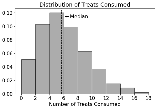
Select the answer closest to the mean of "treats".
4
7
12
Answer: 7
The average score on this problem was 81%.
Select the answer closest to the standard deviation of
"treats".
1
4
16
Answer: 4
The average score on this problem was 85%.
You compute the following statistics about the
"top_speed" column:
mean = 14.6
median = 16.3
You also know that no cat ran at a top speed of exactly 14.6 or 16.3 miles per hour. Select all true statements.
Exactly half of the cats had a top speed greater than 16.3 miles per hour.
There must be at least one cat with a top speed between 14.6 and 16.3 miles per hour.
The output of
(cats.get("top_speed") - 16.3).sum() > 0 is
True.
If we were to add a row to cats for a cat with a top
speed of 20 miles per hour, the median
must increase.
None of the above.
Answer: Options 1 and 4.
The average score on this problem was 73%.
According to Chebyshev’s inequality, at least 80% of San Diego apartments have a monthly parking fee that falls between $30 and $70.
What is the average monthly parking fee?
Answer: \$50
We are given that the left and right bounds of Chebyshev’s inequality are $30 and $70 respectively. Thus, to find the middle of the two, we compute the following equation (the midpoint equation):
\frac{\text{right} + \text{left}}{2}
\frac{70 + 30}{2} = 50
Therefore, 50 is the average monthly parking fee.
The average score on this problem was 92%.
What is the standard deviation of monthly parking fees?
\frac{20}{\sqrt{5}}
\frac{40}{\sqrt{5}}
20\sqrt{5}
20\sqrt{5}
Answer: \frac{20}{\sqrt{5}}
Chebyshev’s inequality states that at least 1 - \frac{1}{z^2} of values are within z standard deviations of the mean. In addition, z can be represented as \frac{\text{bound} - \text{mean of x}}{\text{SD of x}}.
Therefore, we can set up the equation like so: \frac{4}{5} = 1 - \frac{1}{(\frac{\text{bound} - \text{mean of x}}{\text{SD of x}})^2}
Then, we can solve: \frac{1}{5} = \frac{1}{(\frac{\text{bound} - \text{mean of x}}{\text{SD of x}})^2}
Now since we know both bounds, we can plug one of them in. Since the mean was computed in the earlier step, we also plug this in.
\frac{1}{5} = \frac{1}{(\frac{70 - 50}{\text{SD of x}})^2} 5 = (\frac{20}{\text{SD of x}})^2 \sqrt{5} = \frac{20}{\text{SD of x}} \text{SD of x} = \frac{20}{\sqrt{5}}
The average score on this problem was 70%.
The DataFrame restaurants contains information about a
sample of restaurants in San Diego County. We have each restaurant’s
"name" (str), "rating" (int), average
"meal_price" (float), and type of
"cuisine" (str), such as "Thai" or
"Italian".
You are interested in estimating the average
"meal_price" across all Italian restaurants in San Diego
County using only the data in restaurants. Fill in the
following code so that italian_means evaluates to an array
of 1000 bootstrapped estimates for this parameter.
    def bootstrap_means(data, n_samples):
        means = np.array([])
        for i in range(n_samples):
            resample = data.sample(__(a)__, replace = __(b)__)
            means = np.append(means, __(c)__)
        return means

    italian_restaurants = __(d)__
italian_means = bootstrap_means(italian_restaurants, __(e)__)(a): data.shape[0]
(b): True
(c): resample.get("meal_price").mean()
(d):
restaurants[restaurants.get("cuisine") == "Italian"]
(e): 1000
The average score on this problem was 73%.
Next, fill in the blanks below so that italian_CI
evaluates to an 88% bootstrapped confidence interval for the average
"meal_price" across all Italian restaurants in San Diego
County.
    lower_bound = np.percentile(italian_means, __(a)__)
    upper_bound = np.percentile(italian_means, __(b)__)
italian_CI = [lower_bound, upper_bound](a): 6
(b): 94
The average score on this problem was 83%.
Suppose italian_CI evaluates to [25, 35]. Which of the
following statements are correct? Select all that apply.
If we randomly selected 1000 Italian restaurants from the population
of Italian restaurants in San Diego County, about 880 of them will have
an average "meal_price" between $25 and $35.
There is an 88% chance that the average "meal_price" of
Italian restaurants in San Diego County falls between $25 and $35.
88% of all Italian restaurants have an average
"meal_price" between $25 and $35.
None of the above.
Option 4: None of the above.
The average score on this problem was 64%.
In an annual ceremony known as the reaping, tributes are selected to represent their district in the Hunger Games. One male and one female tribute from each district are randomly selected via a lottery drawing.
Every child between the ages of 12 and 18 (inclusive) has tickets entered into the drawing for their sex and district (e.g. girls from District 12). The number of tickets entered is dependent on age.
Starting at age 12, each child receives one ticket in the lottery. For each year after that, they receive one additional ticket, added to the total from the previous year. For example, 13-year-olds have two tickets, 14-year-olds have three tickets, and so on.
In this problem, we will consider only tickets corresponding to girls from District 12, and look at the distribution of these tickets according to the age of the person they represent. A density histogram for these tickets is shown below.
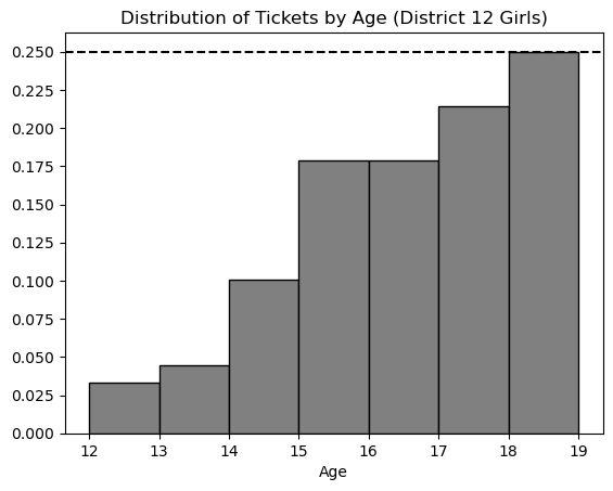
Which of the following statements about this distribution is correct?
The mean is less than the median.
The mean is the same as the median.
The mean is greater than the median.
It is impossible to determine the relationship between the mean and
Answer: The mean is less than the median
The histogram shows us that most of the tickets are for older girls i.e. girls that are of ages 17 to 19. It also shows us that there are fewer tickets for the younger girls. When most of the values are larger, the median is larger than the mean because the small values tend to pull the mean down.
The average score on this problem was 70%.
The histogram from the previous page is repeated below for your reference.
Suppose the rules of the Hunger Games were changed to eliminate 18-year-olds. If we plotted a new density
histogram of the distribution of ages for tickets corresponding to girls
from District 12 aged 12 to 17, how would the height of the
[13, 14) bar change?
Let h be the height of this bar in the original histogram. Give its height in the new histogram in terms of h.
Answer: 4/3 * h
The total area under a density histogram is 1. Using this bit of information, when the 18 year olds are removed we have to scale the the remaining bars so that the area of our density histogram is still 1. Notice the height of the exempt bar is 0.25 meaning that the remaining data is exactly 3/4 th of the original data. To rescale we need to divide the height h of each bar by 3/4 or multiply h by 4/3.
The average score on this problem was 40%.
What is the most common age among girls from District 12 aged 12 to 18? Remember, the distribution above is for all tickets, and older girls have more tickets.
12
13
14
15
16
17
18
Answer: 15
For this problem we need to calculate which bar has the most amount of girls within the bar keeping in mind that each age group gets a different amount of tickets. To do this we can calculate the proportion of girls in each bar relative to the total ticket distribution by dividing the height of each bar by the number of tickets allocated to that bar. The bar for age 15 comes out to the largest with a value of 0.045, and therefore that is our solution.
The average score on this problem was 75%.
The night before the Hunger Games begins, each tribute is interviewed in front of a live audience. During this interview, the host asks each tribute a few personal questions and reveals their overall score from the training camp. These interviews are broadcast across the country, so that the residents of Panem can get to know the tributes better and form opinions about who they want to win.
The Capitol wants to understand public perceptions of the tributes after the interviews for the 74th Hunger Games. They conduct a survey of a sample of residents from all 12 districts, asking them two questions:
“What district do you live in?"
“Who do you think will win this year’s Hunger Games?"
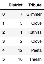
The survey results are in the DataFrame survey, with
columns "District" and "Tribute" which contain
each person’s answers to the two questions above. The first few rows of
survey are shown below.
In this problem, we will try to estimate the proportion of residents from a given district who think a certain tribute will win the Hunger Games.
What proportion of residents in District 11 think Peeta will win?
Write one line of code that evaluates to this
proportion in our sample, based on the data in
survey.
Answer:
survey[(survey.get("Tribute") == "Peeta") & (survey.get("District") == 11)].shape[0] / survey[survey.get("District") == 11].shape[0]
This question is just a whole lot of querying. For the numerator we want all the people who answered the survey who are from district 11 and votes for Peeta. We can do this by querying on those two conditions and taking the shape. For the denominator we want all the people from district 11 who answered the survey, so we query for that in the denominator and take the shape.
The average score on this problem was 78%.
Next, we want to create a 95% confidence interval for the proportion
of all residents from a given district who think a
certain tribute will win. Fill in the blanks in the function
win_CI below. This function takes the name of a tribute and
the number of a district and returns the endpoints of a 95% bootstrapped
confidence interval for the proportion of all residents of that district
who think that tribute will win, based on the data in
survey.
For example win_ci("Peeta", 11) returns the endpoints of
a 95% confidence interval for the proportion of all residents from
District 11 who think Peeta will win.
def win_ci(tribute, district):
            only_district = survey[survey.get("District") == district]
            props = np.array([])
            for i in np.arange(10000):
                resample = __(a)__
                tribute_count = __(b)__
                boot_prop = tribute_count / __(c)__
                props = np.append(props, boot_prop)
return [np.percentile(props, 2.5), np.percentile(props, 97.5)](a):
only_district.sample(only_district.shape[0], replace=True)
For the first blank we have to create a bootstrapped sample from just
the rows in the given district. We sample with replacement here as we do
when we bootstrap to keep the same number of rows. That being said we
use the .sample function with replacement to get our sample
from the only_district dataframe containing the rows in the
given district. Within our sample we want the number of rows to be the
same size as the only_district dataframe. so we set the
size argument to be only_district.shape[0].
(b):
resample[resample.get("Tribute") == tribute].shape[0]
Now we want to find how many times the given tribute appears in the
bootstrapped sample. To do that we query the dataframe for the given
tribute and the take the size of our query using
.shape[0].
(c): resample.shape[0]
The denominator of our resample is just the total number of people in
the resample. That being said to fill this blank all we need to do is
use .shape[0] to take the size of the resample.
The average score on this problem was 59%.
Suppose we were to plot a histogram of props within the
function win_CI. Which of the following best describes this
histogram?
The histogram reflects the shape of the population.
The histogram reflects the shape of the data in
survey.
The histogram reflects the shape of the data in survey
which corresponds to the given district.
The histogram is roughly normal because of the Central Limit Theorem (CLT).
The histogram is roughly normal, but not because of the CLT.
Answer: The histogram is roughly normal because of the Central Limit Theorem (CLT).
The props histogram shows the ditribution of proportions from a bunch of random resamples. Per the CLT, the distribution of sample stats like proportions will be basically normal, regardless of the shape of the original dataset.
The average score on this problem was 53%.
Suppose we now compute the following:
win_ci("Katniss", 4)
[0.25, 0.72]
win_ci("Katniss", 12)
[0.50, 0.70]
Which of the following reasons best explains why the second interval is narrower than the first?
More people live in District 12 than District 4.
More people live in District 4 than District 12.
A greater fraction of District 12 residents than District 4 residents think Katniss will win.
A greater fraction of District 4 residents than District 12 residents think Katniss will win.
There are more survey participants from District 12 than District 4.
There are more survey participants from District 4 than District 12.
Answer: There are more survey participants from District 12 than District 4.
Confidence intervals get narrower when there is an increase in sample size. This is because the variation present in the bootstrapped estimates is smaller. Therefore, we can say there were more survey participants from District 12 than District 4.
The average score on this problem was 68%.
Suppose we want to redo our survey so that our confidence interval for the proportion of District 12 residents who think Katniss will win has a width of at most 0.10. We will assume that our new sample’s standard deviation will be the same as our original sample’s standard deviation. Which of the following best describes how to achieve this?
Our new sample should have twice as many people from District 12. It doesn’t matter how many people the sample contains overall.
Our new sample should have four times as many people from District 12. It doesn’t matter how many people the sample contains overall.
Our new sample should have twice as many people overall. It doesn’t matter how many of them are from District 12.
Our new sample should have four times as many people overall. It doesn’t matter how many of them are from District 12.
Answer: Our new sample should have four times as many people from District 12. It doesn’t matter how many people the sample contains overall.
The width of a confidence interval gets smaller as we collect more data, and it shrinks proportional to \frac{1}{\sqrt{n}}, where n is the sample size.
If we want the interval to be half as wide, we need \frac{1}{\sqrt{n}} to be cut in half, which means n must become four times as large:
\frac{1}{\sqrt{n_{\text{new}}}} = \frac{1}{\sqrt{4n}} = \frac{1}{2\sqrt{n}} \;\Longrightarrow\; n_{\text{new}} = 4n.
The average score on this problem was 75%.
The data visualization below shows all Olympic gold medals for women’s gymnastics, broken down by the age of the gymnast.
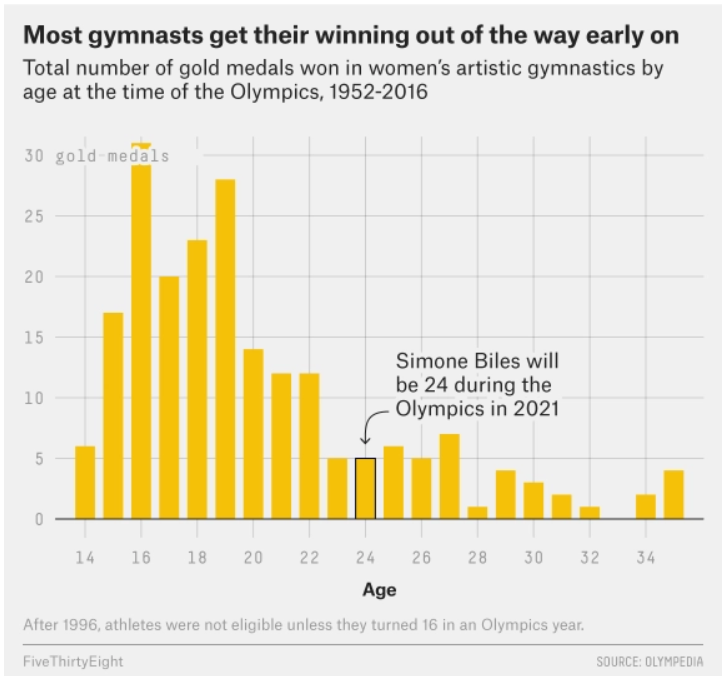
Based on this data, rank the following three quantities in ascending order: the median age at which gold medals are earned, the mean age at which gold medals are earned, the standard deviation of the age at which gold medals are earned.
mean, median, SD
median, mean, SD
SD, mean, median
SD, median, mean
Answer: SD, median, mean
The standard deviation will clearly be the smallest of the three
values as most of the data is encompassed between the range of
[14-26]. Intuitively, the standard deviation will have to
be about a third of this range which is around 4 (though this is not the
exact standard deviation, but is clearly much less than the mean and
median with values closer to 19-25). Comparing the median and mean, it
is important to visualize that this distribution is skewed right. When
the data is skewed right it pulls the mean towards a higher value (as
the higher values naturally make the average higher). Therefore, we know
that the mean will be greater than the median and the ranking is SD,
median, mean.
The average score on this problem was 72%.
Which of the following is larger for this dataset?
the difference between the 50th percentile of ages and the 25th percentile of ages
the difference between the 75th percentile of ages and the 50th percentile of ages
both are the same
Answer: the difference between the 75th percentile of ages and the 50th percentile of ages
Since the distribution is right skewed, the 75th percentile will have a larger difference from the 50th percentile than the 25th percentile. With right skewness, values above the 50th percentile will be more different than those smaller than the 50th percentile (and thus more spread out according to the graph).
The average score on this problem was 78%.
Select all the true statements below.
The average of the deviations from the mean is a meaningful measure of the spread of the data.
It is possible for the standard deviation of a dataset to equal zero.
It is possible for the standard deviation of a dataset to be negative.
Given the standard deviation of a dataset, we can determine its mean.
Given the standard deviation of a dataset, we can determine its variance.
Answer: Option 2 and Option 5
The average score on this problem was 80%.