← return to practice.dsc10.com
Below are practice problems tagged for Lecture 16 (rendered directly from the original exam/quiz sources).
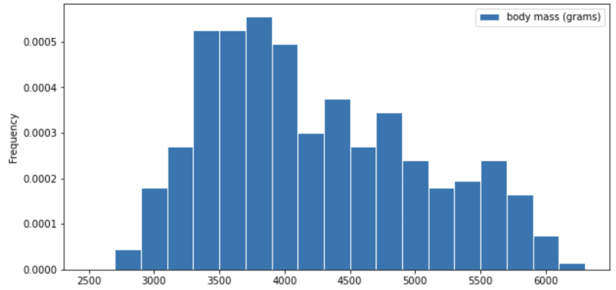
Researchers from the San Diego Zoo, located within Balboa Park, collected physical measurements of several species of penguins in a region of Antarctica.
One piece of information they tracked for each of 330 penguins was its mass in grams. The average penguin mass is 4200 grams, and the standard deviation is 840 grams.
Consider the histogram of mass below.
Select the true statement below.
The median mass of penguins is larger than the average mass of penguins
The median mass of penguins is roughly equal to the average mass of penguins (within 50 grams)
The median mass of penguins is less than the average mass of penguins
It is impossible to determine the relationship between the median and average mass of penguins just by looking at the above histogram
Answer: The median mass of penguins is less than the average mass of penguins
This is a distribution that is skewed to the right, so mean is greater than median.
The average score on this problem was 87%.
Which of the following is a valid conclusion that we can draw solely from the histogram above?
The number of penguins with a mass of exactly 3500 grams is greater than the number of penguins with a mass of exactly 5500 grams.
The number of penguins with a mass of at most 3500 grams is greater than the number of penguins with a mass of at least 5500 grams.
There is an odd number of penguins in the dataset.
The number penguins with a mass of exactly 4000 grams is greater than zero.
None of the above.
Answer: The number of penguins with a mass of at most 3500 grams is greater than the number of penguins with a mass of at least 5500 grams.
Recall, a histogram has intervals on the axis, so we cannot know the frequency of an exact value. Thus, we cannot conclude statements 1, 3, 4. Since the frequency of an exact value is unknown, for statement 3, it is possible that all numbers we have in this distribution are even. Although in the graph, we are only given frequency rather than number, we can justify statement 2 by comparing the area in the left side of 3500, and the area in the right side of 5500. You can either estimate by visually comparing the areas of both parts or compute the area sum of both sides by estimating the bars’ height and windth.
The average score on this problem was 89%.
For your convenience, we show the histogram of mass again below.
Recall, there are 330 penguins in our dataset. Their average mass is 4200 grams, and the standard deviation of mass is 840 grams.
Per Chebyshev’s inequality, at least what percentage of penguins have a mass between 3276 grams and 5124 grams? Input your answer as a percentage between 0 and 100, without the % symbol. Round to three decimal places.
Answer: 17.355
Recall, Chebyshev’s inequality states that No matter what the shape of the distribution is, the proportion of values in the range “average ± z SDs” is at least 1 - \frac{1}{z^2}.
To approach the problem, we’ll start by converting 3276 grams and 5124 grams to standard units. Doing so yields \frac{3276 - 4200}{840} = -1.1, similarly, \frac{5124 - 4200}{840} = 1.1. This means that 3276 is 1.1 standard deviations below the mean, and 5124 is 1.1 standard deviations above the mean. Thus, we are calculating the proportion of values in the range “average ± 1.1 SDs”.
When z = 1.1, we have 1 - \frac{1}{z^2} = 1 - \frac{1}{1.1^2} \approx 0.173553719, which as a percentage rounded to three decimal places is 17.355\%.
The average score on this problem was 76%.
Per Chebyshev’s inequality, at least what percentage of penguins have a mass between 1680 grams and 5880 grams?
50%
55.5%
65.25%
68%
75%
88.8%
95%
Answer: 75%
Recall: proportion with z SDs of the mean
| Percent in Range | All Distributions (via Chebyshev’s Inequality) | Normal Distributions |
|---|---|---|
| \text{average} \pm 1 \ \text{SD} | \geq 0\% | \approx 68\% |
| \text{average} \pm 2\text{SDs} | \geq 75\% | \approx 95\% |
| \text{average} \pm 3\text{SDs} | \geq 88\% | \approx 99.73\% |
To approach the problem, we’ll start by converting 3276 grams and 5124 grams to standard units. Doing so yields \frac{1680 - 4200}{840} = -3, similarly, \frac{5880 - 4200}{840} = 2. This means that 1680 is 3 standard deviations below the mean, and 5880 is 2 standard deviations above the mean.
Proportion of values in [-3 SUs, 2 SUs] >= Proportion of values in [-2 SUs, 2 SUs] >= 75% (Since we cannot assume that the distribution is normal, we look at the All Distributions (via Chebyshev’s Inequality) column for proportion).
Thus, at least 75% of the penguins have a mass between 1680 grams and 5880 grams.
The average score on this problem was 72%.
The distribution of mass in grams is not roughly normal. Is the distribution of mass in standard units roughly normal?
Yes
No
Impossible to tell
Answer: No
The shape of the distribution does not change since we are scaling the x values for all data.
The average score on this problem was 60%.
Suppose all 330 penguin body masses (in grams) that the researchers
collected are stored in an array called masses. We’d like
to estimate the probability that two different randomly selected
penguins from our dataset have body masses within 50 grams of one
another (including a difference of exactly 50 grams). Fill in the
missing pieces of the simulation below so that the function
estimate_prob_within_50g returns an estimate for this
probability.
def estimate_prob_within_50g():
    num_reps = 10000
    within_50g_count = 0
    for i in np.arange(num_reps):
        two_penguins = np.random.choice(__(a)__)
        if __(b)__:
            within_50g_count = within_50g_count + 1
    return within_50g_count / num_reps
What goes in blank (a)? What goes in blank (b)?
Answer: (a) masses, 2, replace=False
(b) abs(two_penguins[0] - two_penguins[1])<=50
np.random.choice( ) can have three parameters
array, n, replace=False, and returns n elements from the
array at random, without replacement. We are randomly choosing 2
different penguins from the masses
array, so we are using np.random.choice( )
without replacement.two_penguins and
calculating their absolute difference with abs(). And in
this if condition, we only want to have penguins with
absolute difference less than or equal to 50, so we write a
<= condition to justify whether the generated pairs of
penguins fulfill this requirement.
The average score on this problem was 84%.
Recall, there are 330 penguins in our dataset. Their average mass is 4200 grams, and the standard deviation of mass is 840 grams. Assume that the 330 penguins in our dataset are a random sample from the population of all penguins in Antarctica. Our sample gives us one estimate of the population mean.
To better estimate the population mean, we bootstrapped our sample and plotted a histogram of the resample means, then took the middle 68 percent of those values to get a confidence interval. Which option below shows the histogram of the resample means and the confidence interval we found?
Option 1
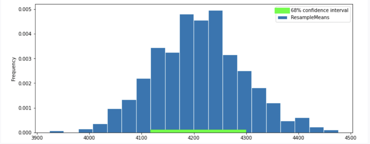
Option 2
Option 3
Option 4
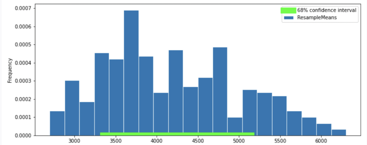
Answer: Option 2
Recall, according to the Central Limit Theorem (CLT), the probability distribution of the sum or mean of a large random sample drawn with replacement will be roughly normal, regardless of the distribution of the population from which the sample is drawn.
Thus, our graph should have a normal distribution. We eliminate Option 4.
Recall that the standard normal curve has inflection points at z = +-1, which is 68% proportion of a normal distribution.(inflection point is where a curve goes from “opening down” to “opening up”) Since we have a confidence intervel of 68% in this question, by looking at the inflection point, we can eliminate Option 3
To compute the SD of the sample mean’s distribution, when we don’t know the population’s SD, we can use the sample’s SD (840): \text{SD of Distribution of Possible Sample Means} \approx \frac{\text{Sample SD}}{\sqrt{\text{sample size}}} = \frac{840}{\sqrt{330}} \approx 46.24
Recall: proportion with z SDs of the mean
| Percent in Range | All Distributions (via Chebyshev’s Inequality) | Normal Distributions |
|---|---|---|
| \text{average} \pm 1 \ \text{SD} | \geq 0\% | \approx 68\% |
| \text{average} \pm 2\text{SDs} | \geq 75\% | \approx 95\% |
| \text{average} \pm 3\text{SDs} | \geq 88\% | \approx 99.73\% |
In this question, we want 68% confidence interval, given that the distribution of sample mean is roughly normal, our CI should have range \text{sample mean} \pm 1 \ \text{SD}. Thus, the interval is approximately [4200-46.24 = 4153.76, 4200+46.24=4246.24]. We compare the 68% CI in Option 1, 2 and we choose Option 2 since it has a 68% CI with approximately the same interval.
The average score on this problem was 66%.
Suppose boot_means is an array of the resampled means.
Fill in the blanks below so that [left, right] is a 68%
confidence interval for the true mean mass of penguins.
left = np.percentile(boot_means, __(a)__)
right = np.percentile(boot_means, __(b)__)
[left, right]
What goes in blank (a)? What goes in blank (b)?
Answer: (a) 16 (b) 84
Recall, np.percentile(array, p) computes the
pth percentile of the numbers in array. To
compute the 68% CI, we need to know the percentile of left tail and
right tail.
left percentile = (1-0.68)/2 = (0.32)/2 = 0.16 so we have 16th percentile
right percentile = 1-((1-0.68)/2) = 1-((0.32)/2) = 1-0.16 = 0.84 so we have 84th percentile
The average score on this problem was 94%.
Which of the following is a correct interpretation of this confidence interval? Select all that apply.
There is an approximately 68% chance that mean weight of all penguins in Antarctica falls within the bounds of this confidence interval.
Approximately 68% of penguin weights in our sample fall within the bounds of this confidence interval.
Approximately 68% of penguin weights in the population fall within the bounds of this interval.
If we created many confidence intervals using the same method, approximately 68% of them would contain the mean weight of all penguins in Antarctica.
None of the above
Answer: Option 4 (If we created many confidence intervals using the same method, approximately 68% of them would contain the mean weight of all penguins in Antarctica.)
Recall, what a k% confidence level states is that approximately k% of the time, the intervals you create through this process will contain the true population parameter.
In this question, our population parameter is the mean weight of all penguins in Antarctica. So 86% of the time, the intervals you create through this process will contain the mean weight of all penguins in Antarctica. This is the same as Option 4. However, it will be false if we state it in the reverse order (Option 1) since our population parameter is already fixed.
The average score on this problem was 81%.
Suppose variables v1, v2, v3,
and v4, have already been initialized to specific numerical
values. Right now, we don’t know what values they’ve been set to.
The function f shown below takes in a number,
v, and outputs an integer between -2 and 2, depending on
the value of v relative to v1,
v2, v3, and v4.
def f(v):
    if v <= v1:
        return -2
    elif v <= v2:
        return -1
    elif v <= v3:
        return 0
    elif v <= v4:
        return 1
    else:
        return 2
Recall that in the previous problem, we created an array called
sample_means containing 10,000 values, each of which is the
mean of a random sample of 100 applicant ages drawn from the DataFrame
apps, in which ages have a mean of 35 and a standard
deviation of 10.
When we call the function f on every value
v in sample_means, we produce a collection of
10,000 values all between -2 and 2. A density histogram of these values
is shown below.
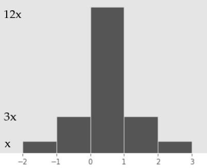
The heights of the five bars in this histogram, reading from left to right, are
x, 3x, 12x, 3x, x.
What is the value of x (i.e. the height of the shortest bar in the histogram)? Give your answer as a fully simplified fraction.
Answer: \frac{1}{20}
In any density histogram, the total area of all bars is 1. This histogram has five bars, each of which has a width of 1 (e.g. 3 - 2 = 1). Since \text{Area} = \text{Height} \cdot \text{Width}, we have that the area of each bar is equal to its height. So, the total area of the histogram in this case is the sum of the heights of each bar:
\text{Total Area} = x + 3x + 12x + 3x + x = 20x
Since we know that the total area is equal to 1, we have
20x = 1 \implies \boxed{x = \frac{1}{20}}
The average score on this problem was 72%.
What does the expression below evaluate to? Give your answer as an integer.
np.count_nonzero((sample_means > v2) & (sample_means <= v4))Hint: Don’t try to find the values of v2 and
v4 – you can answer this question without them!
Answer: 7,500
First, it’s a good idea to understand what the integer we’re trying
to find actually means in the context of the information provided. In
this case, it’s the number of sample means that are greater than
v2 and less than or equal to v4. Here’s how to
arrive at that conclusion:
sample_means is an array of length
10,000.sample_means > v2 and
sample_means <= v4 are both Boolean arrays of length
10,000.(sample_means > v2) & (sample_means <= v4) is
also a Boolean array of length 10,000, which contains True
for every sample mean that is greater than v2 and less than
or equal to v4 and False for every other
sample mean.np.count_nonzero((sample_means > v2) & (sample_means <= v4))
is a number between 0 and 10,000, corresponding to the
number of True elements in the array
(sample_means > v2) & (sample_means <= v4).Remember, the histogram we’re looking at visualizes the distribution
of the 10,000 values that result from calling f on every
value in sample_means. To proceed, we need to understand
how the function f decides what value to return
for a given input, v:
v is greater than v2, then
the first two conditions (v <= v1 and
v <= v2) are False, and so the only
possible values of f(v) are 0, 1,
or 2.v is less than or equal to
v4, the only possible values of f(v) are
-2, -1, 0, 1.v is greater than
v2 and less than or equal to v4, the
only possible values of f(v) are 0 and
1.Now, our job boils down to finding the number of values in the
visualized distribution that are equal to 0 or 1. This is equivalent to
finding the number of values that fall in the [0, 1) and [1,
2) bins – since f only returns integer values, the
only value in the [0, 1) bin is 0 and
the only value in the [1, 2) bin is 1
(remember, histogram bins are left-inclusive and right-exclusive).
To do this, we need to find the proportion of values in those two bins, and multiply that proportion by the total number of values (10,000).
We know that the area of a bar is equal to the proportion of values in that bin. We also know that, in this case, the area of each bar is equal to its height, since the width of each bin is 1. Thus, the proportion of values in a given bin is equal to the height of the corresponding bar. As such, the proportion of values in the [0, 1) bin is 12x, and the proportion of values in the [1, 2) bin is 3x, meaning the proportion of values in the histogram that are equal to either 0 or 1 is 12x + 3x = 15x.
In the previous subpart, we found that x = \frac{1}{20}, so the proportion of values in the histogram that are equal either 0 or 1 is 15 \cdot \frac{1}{20} = \frac{3}{4}*, and since there are 10,000 values being visualized in the histogram total, \frac{3}{4} \cdot 10,000 = 7,500 of them are equal to either 0 or 1.
Thus, 7,500 of the values in sample_means are greater
than v2 and less than or equal to v4, so
np.count_nonzero((sample_means > v2) & (sample_means <= v4))
evaluates to 7,500.
Note: It’s possible to answer this subpart without knowing the value of x, i.e. without answering the previous subpart. The area of the [0, 1) and [1, 2) bars is 15x, and the total area of the histogram is 20x. So, the proportion of the area in [0, 1) or [1, 2) is \frac{15x}{20x} = \frac{15}{20} = \frac{3}{4}, which is the same value we found by substituting x = \frac{1}{20} into 15x.
The average score on this problem was 40%.
Suppose we have run the code below.
from scipy import stats

def g(u):
    return stats.norm.cdf(u) - stats.norm.cdf(-u)
Several input-output pairs for the function g are shown
in the table below. Some of them will be useful to you in answering the
questions that follow.
u | g(u) |
|---|---|
| 0.84 | 0.60 |
| 1.28 | 0.80 |
| 1.65 | 0.90 |
| 2.25 | 0.975 |
What is the value of v3, one of the variables used in
the function f? Give your answer as a number.
Hint: Use the histogram as well as one of the rows of the table above.
Answer: 35.84
The table provided above tells us the proportion of values within u standard deviations of the mean in a normal distribution, for various values of u. For instance, it tells us that the proportion of values within 1.28 standard deviations of the mean in a normal distribution is 0.8.
Let’s reflect on what we know at the moment:
f returns 0 for all inputs that are
greater than v2 and less than or equal to v3.
This, combined with the fact above, tells us that the proportion
of sample means between v2 (exclusive) and v3
(inclusive) is 0.6.Combining the facts above, we have that v2 is 0.84
standard deviations below the mean of the sample mean’s distribution and
v3 is 0.84 standard deviations above the mean of the sample
mean’s distribution.
The sample mean’s distribution has the following characteristics:
\begin{align*} \text{Mean of Distribution of Possible Sample Means} &= \text{Population Mean} = 35 \\ \text{SD of Distribution of Possible Sample Means} &= \frac{\text{Population SD}}{\sqrt{\text{Sample Size}}} = \frac{10}{\sqrt{100}} = 1 \end{align*}
0.84 standard deviations above the mean of the sample mean’s distribution is:
35 + 0.84 \cdot \frac{10}{\sqrt{100}} = 35 + 0.84 \cdot 1 = \boxed{35.84}
So, the value of v3 is 35.84.
The average score on this problem was 9%.
Which of the following is closest to the value of the expression below?
np.percentile(sample_means, 5)14
14.75
33
33.35
33.72
Answer: 33.35
The table provided tells us that in a normal distribution, 90% of values are within 1.65 standard deviations of the mean. Since normal distributions are symmetric, it also means that 5% of values are above 1.65 standard deviations of the mean and, more importantly, 5% of values are below 1.65 standard deviations of the mean.
The 5th percentile of a distribution is the smallest value that is
greater than or equal to 5% of values, so in this case the 5th
percentile is 1.65 SDs below the mean. As in the previous subpart, the
mean and SD we are referring to are the mean and SD of the distribution
of sample means (sample_means), which we found to be 35 and
1, respectively.
1.65 standard deviations below this mean is
35 - 1.65 \cdot 1 = \boxed{33.35}
The average score on this problem was 45%.
On Reddit, Yutian read that 22% of all online transactions are fraudulent. She decides to test the following hypotheses:
Null Hypothesis: The proportion of online transactions that are fraudulent is 0.22.
Alternative Hypothesis: The proportion of online transactions that are fraudulent is not 0.22.
To test her hypotheses, she decides to create a 95% confidence interval for the proportion of online transactions that are fraudulent using the Central Limit Theorem.
Unfortunately, she doesn’t have access to the entire txn
DataFrame; rather, she has access to a simple random sample of
txn of size n. In her
sample, the proportion of transactions that are fraudulent is
0.2 (or equivalently, \frac{1}{5}).
The width of Yutian’s confidence interval is of the form \frac{c}{5 \sqrt{n}}
where n is the size of her sample and c is some positive integer. What is the value of c? Give your answer as an integer.
Hint: Use the fact that in a collection of 0s and 1s, if the proportion of values that are 1 is p, the standard deviation of the collection is \sqrt{p(1-p)}.
Answer: 8
First, we can calculate the standard deviation of the sample using the given formula: \sqrt{0.2\cdot(1-0.2)} = \sqrt{0.16}= 0.4. Additionally, we know that the width of a 95% confidence interval for a population mean (including a proportion) is approximately \frac{4 * \text{sample SD}}{\sqrt{n}}, since 95% of the data of a normal distribution falls within two standard deviations of the mean on either side. Now, plugging the sample standard deviation into this formula, we can set this expression equal to the given formula for the width of the confidence interval: \frac{c}{5 \sqrt{n}} = \frac{4 * 0.4}{\sqrt{n}}. We can multiply both sides by \sqrt{n}, and we’re left with \frac{c}{5} = 4 * 0.4. Now, all we have to do is solve for c by multiplying both sides by 5, which gives c = 8.
The average score on this problem was 59%.
There is a positive integer J such that:
If n < J, Yutian will fail to reject her null hypothesis at the 0.05 significance level.
If n > J, Yutian will reject her null hypothesis at the 0.05 significance level.
What is the value of J? Give your answer as an integer.
Answer: 1600
Here, we have to use the formula for the endpoints of the 95% confidence interval to see what the largest value of n is such that 0.22 will be contained in the interval. The endpoints are given by \text{sample mean} \pm 2 * \frac{\text{sample SD}}{\sqrt{n}}. Since the null hypothesis is that the proportion is 0.22 (which is greater than our sample mean), we only need to work with the right endpoint for this question. Plugging in the values that we have, the right endpoint is given by 0.2 + 2 * \frac{0.4}{\sqrt{n}}. Now we must find a value of n which satisfies the inequality 0.2 + 2 * \frac{0.4}{\sqrt{n}} \geq 0.22, and since we’re looking for the smallest such value of n (i.e, the last n for which this inequality holds), we can simply set the two sides equal to each other, and solve for n. From 0.2 + 2 * \frac{0.4}{\sqrt{n}} = 0.22, we can subtract 0.2 from both sides, then multiply both sides by \sqrt{n}, and divide both sides by 0.02 (from 0.22 - 0.2). This yields \sqrt{n} = \frac{2 * 0.4}{0.02} = \sqrt{n} = 40, which implies that n is 1600.
The average score on this problem was 21%.
At least what proportion of summer.get("students") is in
the range [30,40]?
\geq 0.75
\geq 0.68
\geq 0.25
\geq 0.00
Answer: \geq 0.00
The average score on this problem was 66%.
Ryan runs the code below to make a single array with the contents of
the "students" columns from both summer and
fall.
combined = np.append(summer.get("students"), fall.get("students"))Select all of the true statements below:
The mean of combined is 220.
The mean of combined is in the range (40,400).
The standard deviation of combined is less than 10.
The standard deviation of combined is greater than
10.
None of the above.
Answer: Options 2 and 4.
The average score on this problem was 83%.
Since he was in a rush, Ryan asked ChatGPT to write code that
standardizes combined. To his surprise, 90\% of the standardized data is
less than 0. Which of the following best explains this situation?
Ryan should be surprised; this must have incorrectly standardized the data.
Ryan should be surprised; a number of students cannot be negative.
Ryan should not be surprised; it’s possible for 100\% of the data to be below 0.
Ryan should not be surprised; his data is skewed.
Answer: Option 4.
The average score on this problem was 66%.
For this question only, suppose we know that
summer.get("students") is normally distributed. You
randomly select one number from summer.get("students").
Using the function scipy.stats.norm.cdf, write one
line of code that evaluates to the probability that the number
you selected is in the range [30,45].
Answer:
scipy.stats.norm.cdf(0.5) - scipy.stats.norm.cdf(-1)
The average score on this problem was 55%.
An IKEA chair designer is experimenting with some new ideas for armchair designs. She has the idea of making the arm rests shaped like bell curves, or normal distributions. A cross-section of the armchair design is shown below.
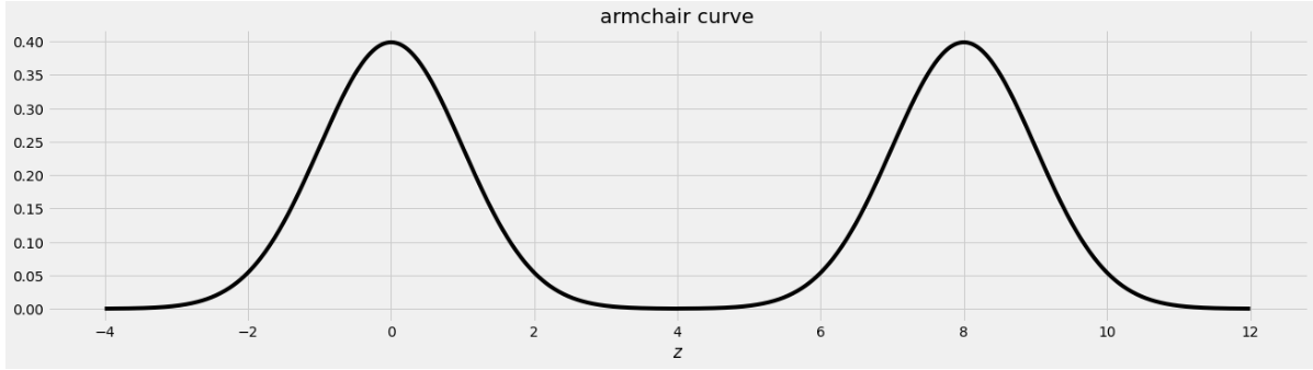
This was created by taking the portion of the standard normal distribution from z=-4 to z=4 and adjoining two copies of it, one centered at z=0 and the other centered at z=8. Let’s call this shape the armchair curve.
Since the area under the standard normal curve from z=-4 to z=4 is approximately 1, the total area under the armchair curve is approximately 2.
Complete the implementation of the two functions below:
area_left_of(z) should return the area under the
armchair curve to the left of z, assuming
-4 <= z <= 12, andarea_between(x, y) should return the area under the
armchair curve between x and y, assuming
-4 <= x <= y <= 12.import scipy
def area_left_of(z):
'''Returns the area under the armchair curve to the left of z.
Assume -4 <= z <= 12'''
if ___(a)___:
return ___(b)___
return scipy.stats.norm.cdf(z)
def area_between(x, y):
'''Returns the area under the armchair curve between x and y.
Assume -4 <= x <= y <= 12.'''
return ___(c)___What goes in blank (a)?
Answer: z>4 or
z>=4
The body of the function contains an if statement
followed by a return statement, which executes only when
the if condition is false. In that case, the function
returns scipy.stats.norm.cdf(z), which is the area under
the standard normal curve to the left of z. When
z is in the left half of the armchair curve, the area under
the armchair curve to the left of z is the area under the
standard normal curve to the left of z because the left
half of the armchair curve is a standard normal curve, centered at 0. So
we want to execute the return statement in that case, but
not if z is in the right half of the armchair curve, since
in that case the area to the left of z under the armchair
curve should be more than 1, and scipy.stats.norm.cdf(z)
can never exceed 1. This means the if condition needs to
correspond to z being in the right half of the armchair
curve, which corresponds to z>4 or z>=4,
either of which is a correct solution.
The average score on this problem was 72%.
What goes in blank (b)?
Answer:
1+scipy.stats.norm.cdf(z-8)
This blank should contain the value we want to return when
z is in the right half of the armchair curve. In this case,
the area under the armchair curve to the left of z is the
sum of two areas:
z.Since the right half of the armchair curve is just a standard normal
curve that’s been shifted to the right by 8 units, the area under that
normal curve to the left of z is the same as the area to
the left of z-8 on the standard normal curve that’s
centered at 0. Adding the portion from the left half and the right half
of the armchair curve gives
1+scipy.stats.norm.cdf(z-8).
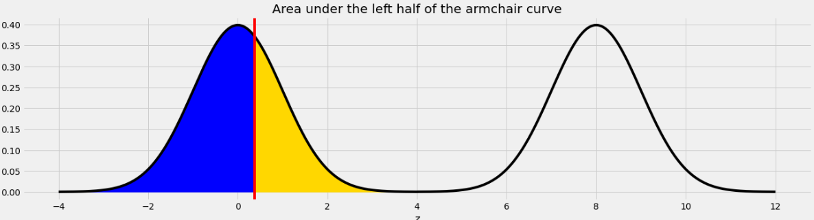
For example, if we want to find the area under the armchair curve to the left of 9, we need to total the yellow and blue areas in the image below.
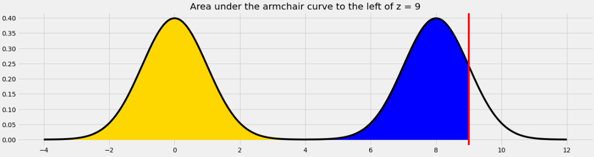
The yellow area is 1 and the blue area is the same as the area under the standard normal curve (or the left half of the armchair curve) to the left of 1 because 1 is the point on the left half of the armchair curve that corresponds to 9 on the right half. In general, we need to subtract 8 from a value on the right half to get the corresponding value on the left half.
The average score on this problem was 54%.
What goes in blank (c)?
Answer:
area_left_of(y) - area_left_of(x)
In general, we can find the area under any curve between
x and y by taking the area under the curve to
the left of y and subtracting the area under the curve to
the left of x. Since we have a function to find the area to
the left of any given point in the armchair curve, we just need to call
that function twice with the appropriate inputs and subtract the
result.
The average score on this problem was 60%.
Suppose you have correctly implemented the function
area_between(x, y) so that it returns the area under the
armchair curve between x and y, assuming the
inputs satisfy -4 <= x <= y <= 12.
Note: You can still do this question, even if you didn’t know how to do the previous one.
What is the approximate value of
area_between(-2, 10)?
1.9
1.95
1.975
2
Answer: 1.95
The area we want to find is shown below in two colors. We can find the area in each half of the armchair curve separately and add the results.
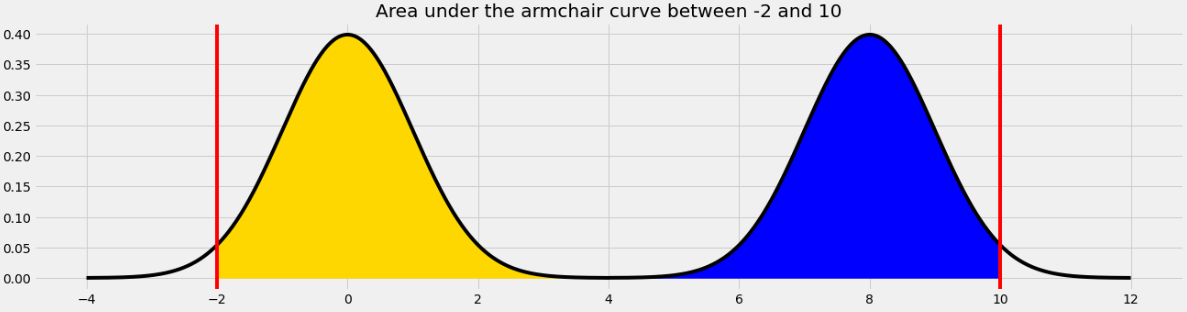
For the yellow area, we know that the area within 2 standard deviations of the mean on the standard normal curve is 0.95. The remaining 0.05 is split equally on both sides, so the yellow area is 0.975.
The blue area is the same by symmetry so the total shaded area is 0.975*2 = 1.95.
Equivalently, we can use the fact that the total area under the armchair curve is 2, and the amount of unshaded area on either side is 0.025, so the total shaded area is 2 - (0.025*2) = 1.95.
The average score on this problem was 76%.
What is the approximate value of
area_between(0.37, 8.37)?
0.68
0.95
1
1.5
Answer: 1
The area we want to find is shown below in two colors.
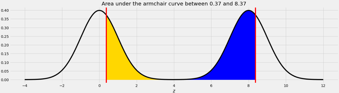
As we saw in Problem 12.2, the point on the left half of the armchair curve that corresponds to 8.37 is 0.37. This means that if we move the blue area from the right half of the armchair curve to the left half, it will fit perfectly, as shown below.
Therefore the total of the blue and yellow areas is the same as the area under one standard normal curve, which is 1.
The average score on this problem was 76%.
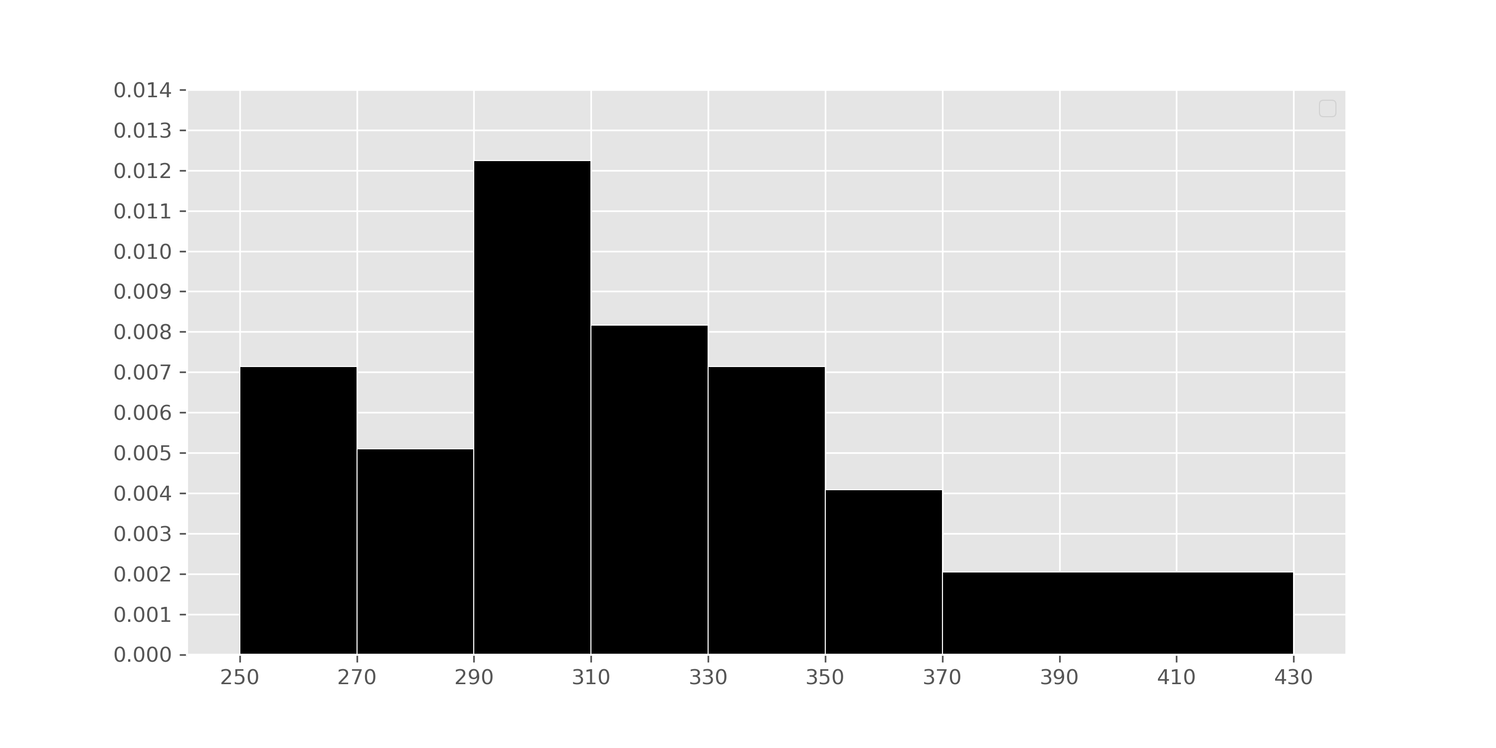
This summer, Zoe wants to explore parts of the United States that she
hasn’t been to yet. In her process of figuring out where to go, she
creates a histogram depicting the distribution of the number of sunshine
hours in July across all cities in the United States in
sun.
Suppose usa is a DataFrame with all of the columns in
sun but with only the rows where "Country" is
"United States".
What is the value of mystery below?
    cond = (usa.get("Jul") >= 370) & (usa.get("Jul") < 430)
    mystery = 100 * np.count_nonzero(cond) / usa.shape[0]
2
8
12
16
18
20
Answer: 12
cond is a Series that contains True for
each row in usa where "Jul" is greater than or
equal to 370 and less than 430. mystery, then, is the
percentage of values in usa in which
cond is True. This is because
np.count_nonzero(cond) is the number of Trues
in cond, np.count_nonzero(cond) / usa.shape[0]
is the proportion of values in cond that are
True, and
100 * np.count_nonzero(cond) / usa.shape[0] is the
percentage of values in cond that are True.
Our goal here, then, is to use the histogram to find the
percentage of values in the histogram between 370 (inclusive) and 430
(exclusive).
We know that in histograms, the area of each bar is equal to the proportion of data points that fall within its bin’s range. Conveniently, there’s only one bar we need to look at – the one corresponding to the bin [370, 430). That bar has a width of 430 - 370 = 60 and a height of 0.002. Then, the area of that bar – i.e. the proportion of values that are between 370 (inclusive) and 430 (exclusive) is:
\text{proportion} = \text{area} = \text{height} \cdot \text{width} = 0.002 \cdot 60 = 0.12
This means that the proportion of values in [370, 430) is 0.12, which
means that the percentage of values in [370, 430) is 12%, and that
mystery evaluates to 12.
The average score on this problem was 83%.
There are 5 more cities with between 370 and 430 sunshine hours in July than there are cities with between 270 and 290 sunshine hours in July.
How many cities in the United States are in sun? Give
your answer as a positive integer, rounded to the nearest multiple of 10
(that is, your answer should end in a 0).
Answer: 250
In the previous part, we learned that the proportion of cities in the
usa DataFrame in the interval [370, 430) (i.e. that have
between 370 and 430 sunshine hours in July) is 0.12. To use the fact
that there are 5 more cities in the interval [370, 430) than there are
in the interval [270, 290), we need to first find the proportion of
cities in the interval [270, 290). To do so, we look at the [270, 290)
bin, which has a width of 290 - 270 =
20 and a height of 0.005:
\text{proportion} = 0.005 \cdot 20 = 0.10
We are told that there are 5 more cities in the [370, 430) interval than there are in the [270, 290) interval. Given the proportions we’ve computed, we have that:
\text{difference in proportions} = 0.12 - 0.1 = 0.02
If 0.02 \cdot \text{number of cities} is 5, then \text{number of cities} = 5 \cdot \frac{1}{0.02} = 5 \cdot 50 = 250.
The average score on this problem was 49%.
Now, suppose we convert the number of sunshine hours in July for all
cities in the United States (i.e., “US cities”) in sun from
their original units (hours) to standard units.
Let m be the mean number of sunshine
hours in July for all US cities in sun, in standard units.
Select the true statement below.
m = -1
-1 < m < 0
m = 0
0 < m < 1
m = 1
m > 1
Answer: m = 0
When we standardize a dataset, the mean of the resulting values is always 0 and the standard deviation of the resulting values is always 1. This tells us right away that the answer is m = 0. Intuitively, we know that a value in standard units represents the number of standard deviations that value is above or below the mean of the column it came from. m is equal to the mean of the column it came from, so m in standard units is 0.
If we’d like to approach this more algebracically, we can remember the formula for converting a value x_i from a column x to standard units:
x_{i \: \text{(su)}} = \frac{x_i - \text{mean of } x}{\text{SD of } x}
Let x be the column (i.e. Series)
containing the mean number of sunshine hours in July for all US cities
in sun. m, by definition,
is the mean of x. Then,
m_{\text{(su)}} = \frac{m - \text{mean of } x}{\text{SD of } x} = \frac{m - m}{\text{SD of }x} = 0
Given that m is the mean of column x, the numerator of m_\text{(su)} is 0, and hence m_\text{(su)} is 0.
The average score on this problem was 62%.
Let s be the standard deviation of
the number of sunshine hours in July for all US cities sun,
in standard units. Select the true statement below.
s = -1
-1 < s <0
s = 0
0 < s < 1
s = 1
s > 1
Answer: s = 1
As mentioned in the previous solution, when we standardize a dataset, the mean of the resulting values is always 0 and the standard deviation of the resulting values is always 1.
The average score on this problem was 46%.
Let d be the median of the number of
sunshine hours in July for all US cities in sun, in
standard units. Select the true statement below.
d = -1
-1 < d < 0
d = 0
0 < d < 1
d = 1
d > 1
Answer: -1 < d <
0
In the histogram, we see that the distribution of the number of
sunshine hours in July for all US cities in sunis skewed
right, or has a right tail. This means that this distribution’s mean is
dragged in the direction of its tail and is larger than its median.
Since the mean in standard units is 0, and the median is less than the
mean, the median in standard units must be negative. There’s no property
that states that the median is exactly -1, and the median is only
slightly less than the mean, which means that it must be the case that
-1 < d < 0.
The average score on this problem was 42%.
True or False: The distribution of the number of sunshine hours in
July for all US cities in sun, in standard units, is
roughly normal.
True
False
Impossible to tell
Answer: False
The original histogram depicting the distribution of the number of sunshine hours in July for all US cities is right-skewed. When data is converted to standard units, the shape of the distribution does not change. Therefore, if the original data is right-skewed, the standardized data will also be right-skewed.
The average score on this problem was 45%.
Australia is in the southern hemisphere, meaning that its summer season is from December through February, when we have our winter. As a result, January is typically one of the sunniest months in Australia!
Arjun is a big fan of the movie Kangaroo Jack and plans on visiting
Australia this January. In doing his research on where to go, he found
the number of sunshine hours in January for the 15 Australian cities in
sun and sorted them in descending
order.
356, 337, 325, 306, 294, 285, 285, 266, 263, 257, 255, 254, 220, 210, 176
Throughout this question, use the mathematical definition of percentiles presented in class.
Note: Parts 1, 2, and 3 of this problem are out of scope; they cover material no longer included in the course. Part 4 is in scope!
What is the 80th percentile of the collection of numbers above?
254
255
294
306
325
337
Answer: 306
First, we need to find the position of the 80th percentile using the rule from class:
h = \left(\frac{80}{100}\right) \cdot 15 = \frac{4}{5} \cdot 15 = 12
Since 12 is an integer, we don’t need to round up, so k = 12. Starting from the right-most number, which is the smallest number and hence position 1 here, the 12th number is 306.
The average score on this problem was 52%.
What is the largest positive integer p such that 257 is the pth percentile of the collection of numbers above?
Answer: 40
The first step is to find the position of 257 in the collection when we start at position 1, which is 6. Since there are 15 values total, this means that 257 is the smallest value that is greater than or equal to 40% of the values.
If we set p to be any number larger than 40, say, 41, then 257 won’t be larger than p\% of the values in the collection; thus, the largest positive integer value of p that makes 257 the pth percentile is 40.
The average score on this problem was 30%.
What is the smallest positive integer p such that 257 is the pth percentile of the collection of numbers above? (Make sure your answer to (c) is smaller than your answer to (b)!)
Answer: 34
Let’s look at the next number down from 257, which is 255. 255 is the 5th number out of 15, so it is the smallest number that is greater than or equal to 33.333% of the values. This means the 33rd percentile is also 255, since 33.333 > 33. However, 255 is not greater than or equal to 34% of the values, which makes the 34th percentile 257. Therefore, 34 is the smallest integer value of p such that the pth percentile is 257.
The average score on this problem was 21%.
Teresa also wants to go to Australia, but can’t take time off work in
January, and so she plans a trip to The Land Down Under (Australia) in
February instead. She finds that the mean number of sunshine hours in
February for all 15 Australian cities in sun is 250, with a
standard deviation of 15.
According to Chebyshev’s inequality, at least what percentage of
Australian cities in sun see between 200 and 300 sunshine
hours in February?
9%
30%
33.3%
91%
95%
99.73%
Answer: 91%
First, we need to find the number of standard deviations above the mean 300 is, and the number of standard deviations below the mean 200 is.
z = \frac{300 - 250}{15} = \frac{50}{15} = \frac{10}{3}
The above equation tells us that 300 is \frac{10}{3} standard deviations above the mean; you can verify that 200 is the same number of standard deviations below the mean. Chebyshev’s inequality tells us the proportion of values within z SDs of the mean is at least 1 - \frac{1}{z^2}, which here is:
1 - \frac{1}{\left(\frac{10}{3}\right)^2} = 1 - \frac{9}{100} = 0.91
The average score on this problem was 43%.
You are given the following information about security deposits for a sample of 400 apartments in the Mission Hills neighborhood of San Diego:
Using the fact that scipy.stats.norm.cdf(-0.8) evaluates
to about 0.21, construct a 58% confidence interval for the mean security
deposit of all Mission Hills apartments. Below, give the endpoints of
your confidence interval, both as integers.
Left endpoint: ____(a)____
Right endpoint: ____(b)____
Answer:
scipy.stats.norm.cdf(-0.8) tells us that from the bounds
of (-\inf, -0.8], the normal
distribution has an area of 0.21.
Therefore, if we take it to the other side from [0.8, \inf), it also has an area of 0.21 due to the symmetrical property of the
normal distribution. This means that the interval between [-0.8, 0.8] has an area of 1 - 0.21 - 0.21 = 0.58: the confidence
interval we are aiming to find.
In the question, we are given the standard deviation of security deposits in a sample, meaning we need to find the standard deviation for the population. To find this, we use the following formula and compute:
\frac{\text{SD of sample}}{\sqrt{\text{sample size}}} = \frac{500}{\sqrt{400}} = \frac{500}{20} = 25.
Now that we have the population standard deviation, we can calculate the endpoints of the confidence interval.
Left endpoint: 2300 - \frac{4}{5} \cdot 25 = 2280
Right endpoint: 2300 + \frac{4}{5} \cdot 25 = 2320
The average score on this problem was 29%.
Suppose that the trees on UCSD’s campus have a mean height of 100 feet and a variance of 36 feet. If the height of a specific tree is 124 feet, what would its height be in standard units for this distribution? Simplify your answer.
Answer: 4
The average score on this problem was 73%.
Let A be the answer to the previous question. Choose the best interpretation of A.
A randomly selected tree on UCSD’s campus has an A percent probability of being at least 124 feet tall.
A 124 foot tree is A times taller than the average tree on UCSD’s campus.
A 124 foot tree is A standard deviations taller than the average tree on UCSD’s campus.
At least 95% of trees on UCSD’s campus have a height within A standard deviations of the mean height.
Answer: A 124 foot tree is A standard deviations taller than the average tree on UCSD’s campus.
The average score on this problem was 84%.
You are told that scipy.stats.norm.cdf(-1.4) evaluates
to 0.08075665923377107. Suppose you have a standard normal
curve with mean at x=0 and standard
deviation 1. What is the area under the curve from x=0 to x=1.4? Give your answer as a number rounded
to 2 decimal places.
Answer: 0.42
The average score on this problem was 57%.
Before getting selected for the Hunger Games, Katniss often spent her days hunting with her friend Gale. Hunting is illegal in Panem, so Katniss and Gale sold their poached game at a black market known as The Hob, always splitting the profits equally, even if one person’s kills were worth more than the other’s.
Suppose Katniss and Gale hunted together three times. The values of
each person’s kills are recorded in katniss_sample and
gale_sample, respectively. Their individual profits are
recorded in average_sample. Calculate the mean and variance
of each of these three samples. Give all of your answers as
integers.
| Sample | Mean | Variance |
|---|---|---|
a.) katniss_sample = [47, 44, 50] |
||
b.) gale_sample = [25, 28, 28] |
||
c.) average_sample = [36, 36, 39] |
Answer:
a.) mean: \frac{47+44+50}{3} = \frac{141}{3} = 47; variance: \frac{(47−47)^2+(44−47)^2+(50−47)^2}{3} =
\frac{(0 + 9 + 9)}{3} = 6
b.) mean: \frac{(25+28+28)}{3} = \frac{81}{3} = 27; variance = \frac{(25−27)^2+(28−27)^2+(28−27)^2}{3} =
\frac{(4 + 1 + 1)}{3} = 2
c.) mean: \frac{(36+36+39)}{3} = \frac{111}{3} = 37; variance: \frac{[(36−37)^2+(36−37)^2+(39−37)^2]}{3} =
\frac{(1 + 1 + 4)}{3} = 2
The average score on this problem was 16%.
Suppose that the value of Katniss’s kills are normally distributed with mean \$50 and SD \$3, and the value of Gale’s kills are independently normally distributed with mean \$30 and SD \$2.
On one hunting trip, Katniss’s kills are worth twice as much as Gale’s, but the value of her kills in standard units is the same as the value of Gale’s kills in standard units. Determine the value of Gale’s kills on this hunting trip. Give your answer as an integer.
Answer: 10
If Katniss’s kills (K) are worth twice Gale’s kills (G) we can say that K = 2G. To get the standardized values of each of their kills we can use the formula:
\frac{\text{Kills on Trip} - \text{Mean Kills for Person}}{\text{Std Kills for Person}}
(This is just the regular standardization formula put in the context of this problem).
Furthermore, we know that their standardized values are equal from the problem statement, so after subtituting values in we get the below equality:
\frac{2G - 50}{3} = \frac{G - 30}{2}
Using some basic cross multiplication we can attempt to solve for G now.
4G - 100 = 3G - 90; G = 10
The average score on this problem was 85%.
Now, suppose that we no longer know whether the distribution of the value of Katniss’s kills is normal. All we know about this distribution is that it has mean \$50 and SD \$3.
Which of the following statements are true? Select all that apply.
It is possible that Katniss’s kills are never valued between \$48 and \$52.
No more than 75\% of Katniss’s kills are between \$44 and \$56 in value.
scipy.stats.norm.cdf(50) gives an approximation for the
fraction of Katniss’s kills that are below \$50 in value.
None of these.
Answer: Choice 1 only
Choice 1 could be correct assuming our distribution is not normal, as there could be some sorta two point distribution that has no area under $47 to $53 meaning that Katniss’s kills are never valued in that range.
Choice 2 is False the range given in this choice encompasses 2 standard deviations. Per Chebyshev if we are 2 stds from the mean, at least 75% of the data must lie in our range, meaning there could be more than 75% of the data in this range.
Choice 3 is False aswell because the norm cdf required the assumption of normality.
Choice 4 is incorrect because the first statement is true.
The average score on this problem was 76%.
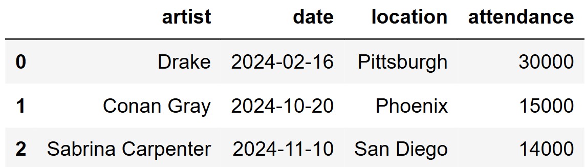
The DataFrame concerts contains data on a sample of
concerts held in 2024. For each concert, we have the name of the
performing "artist", the "date" and
"location" of the concert, and the total
"attendance" as an integer. The first few rows of
concerts are shown below:
You are interested in estimating the average
"attendance" at concerts using the data in
concerts. Fill in the blanks to define a function
estimate_attendance that takes as input a number of
estimates to produce, and returns an array with that number of
bootstrapped estimates of the mean concert attendance.
def estimate_attendance(how_many):
    estimates = np.array([])
    for i in __(a)__:
        resample = ___(b)__
        estimates = np.append(estimates, __(c)__.mean())
return estimates(a): np.arange(how_many)
(b):
concerts.sample(concerts.shape[0], replace=True)
(c): resample.get("attendance")
The average score on this problem was 82%.
Now, fill in the blanks to compute an 85\% confidence interval for the average concert attendance based on 10000 bootstrapped estimates.
boot_attendance = estimate_attendance(__(a)__)
ci_low = np.percentile(boot_attendance, __(b)__)
ci_high = np.percentile(boot_attendance, __(c)__)
concert_interval = [ci_low, ci_high](a): 10000
(b): 7.5
(c): 92.5
The average score on this problem was 90%.
Suppose concert_interval comes out to [18500, 19500]. Which of the following
statements are valid interpretations of this interval? Select all that
apply.
There is an 85\% chance that the average attendance of all concerts is between 18500 and 19500.
85\% of all concerts have an attendance between 18500 and 19500.
If we were to make many different confidence intervals based on different samples of concerts, approximately 85\% of the resulting intervals would contain the true average concert attendance.
None of the above.
Answer: Option 3 only.
The average score on this problem was 84%.
You are told that the data in the "attendance" column of
concerts has a mean of 19000 and a standard deviation of 3000. Find the endpoints of the smallest
interval which is guaranteed to contain at least \frac{15}{16} of the data. Both endpoints
should be given as integers.
Answer: [7000, 31000]
The average score on this problem was 74%.
You are now told that the data in the "attendance"
column is normally distributed. Approximately what percentage of the
data is included in the interval you gave above? Give your answer
to the nearest integer.
Answer: 100
The average score on this problem was 43%.
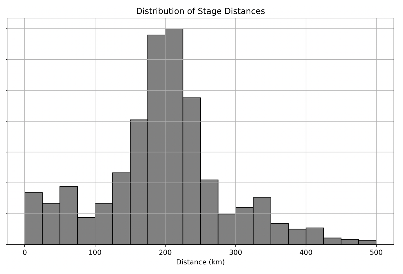
Below is a density histogram representing the distribution of randomly sampled stage distances.
Which statement below correctly describes the relationship between the mean and the median of the sampled stage distances?
The mean is significantly larger than the median.
The mean is significantly smaller than the median.
The mean is approximately equal to the median.
It is impossible to know the relationship between the mean and the median.
Answer: The mean is approximately equal to the median.
The average score on this problem was 55%.
Assume there are 100 stages in the random sample that generated this
plot. If there are 5 stages in the bin [275, 300),
approximately how many stages are in the bin
[200, 225)?
Answer: 35 = 5\cdot7
[200, 225) on the density
histogram is approximately 7 times the height of the
bin [275, 300).[200, 225) is 35 = 5\cdot7.
The average score on this problem was 78%.
Assume the mean distance is 200 km and the standard deviation is 50 km. At least what proportion of stage distances are guaranteed to lie between 0 km and 400 km? Do not simplify your answer.
Answer: \frac{15}{16}
Using Chebyshev’s inequality, we know at least 1 - \frac{1}{z^2} of the data lies within z SDs. Here, z = 4 so we know 1 - \frac{1}{16} = \frac{15}{16} of the data lie in that range.
The average score on this problem was 73%.
Again, assume the mean stage distance is 200 km and the standard deviation is 50 km. Now, suppose we take a random sample of size 25 from the stage distances, calculate the mean stage distance of this sample, and repeat this process 500 times. What proportion of the means that we calculate will fall between 190 km and 210 km? Do not simplify your answer.
Answer: 68%
We know about 68% of values lie within 1 standard deviation of the mean of any normal distribution. The distribution of means of samples of size 25 from this dataset is normally distributed with mean 200km and SD \frac{50}{\sqrt{25}} = 10, so 190km to 210km contains 68% of the values.
The average score on this problem was 55%.
Assume the mean distance is 200 km and the standard deviation is 50 km. Suppose we use the Central Limit Theorem to generate a 95% confidence interval for the true mean distance of all Tour de France stages, and get the interval [190\text{ km}, 210\text{ km}]. Which of the following interpretations of this confidence interval are correct?
95% of Tour de France stage distances fall between 190 km and 210 km.
There is a 95% chance that the true mean distance of all Tour de France stages is between 190 km and 210 km.
We are 95% confident that the true mean distance of all Tour de France stages is between 190 km and 210 km.
Our sample is of size 100.
Our sample is of size 25.
If we collected many original samples and constructed many 95% confidence intervals, then exactly 95% of those intervals would contain the true mean distance.
If we collected many original samples and constructed many 95% confidence intervals, then roughly 95% of those intervals would contain the true mean distance.
Answer: Option 3, Option 4, and Option 7
Option 1:
Incorrect. Confidence intervals describe the
uncertainty in estimating the population mean, not the proportion of
data points. A 95% confidence interval does not imply that 95% of
individual stage distances fall between 190 km and 210 km.
Option 2:
Incorrect. Confidence intervals are based on the
sampling process, not probability. Once the interval is calculated, the
true mean is either inside or outside the interval. We cannot assign a
probability to this.
Option 3:
Correct. This is the standard interpretation of
confidence intervals: “We are 95% confident that the true mean lies
within the interval.”
Option 4:
Correct. Given a sample size of 100 and population
standard deviation of 50, the confidence interval ([190, 210]) is
consistent with the calculation using the rule of thumb that a 95%
confidence interval is approximately 2 standard deviations apart
from the mean.
For a 95% confidence interval, the range can be approximated as:
\left[\text{sample mean} - 2\cdot \frac{\text{sample SD}}{\sqrt{\text{sample size}}}, \text{sample mean} + 2\cdot \frac{\text{sample SD}}{\sqrt{\text{sample size}}} \right]
Substituting the given values:
Option 5:
Incorrect. refer to option 4
Option 6:
Incorrect. The wording “exactly 95%” is overly precise.
In practice, confidence intervals are based on the sampling process, and
we use “approximately” or “roughly” 95%.
Option 7:
Correct. By definition of a confidence interval, if we
repeatedly sampled and constructed 95% confidence intervals, roughly 95%
of them would contain the true mean.
The average score on this problem was 72%.
Suppose we take 500 random samples of size 100 from the stage distances, calculate their means, and draw a histogram of the distribution of these sample means. We label this Histogram A. Then, we take 500 random samples of size 1000 from the stage distances, calculate their means, and draw a histogram of the distribution of these sample means. We label this Histogram B. Fill in the blanks so that the sentence below correctly describes how Histogram B looks in comparison to Histogram A.
“Relative to Histogram A, Histogram B would appear __(i)__ and shifted __(ii)__ due to the __(iii)__ mean and the __(iv)__ standard deviation.”
(i):
thinner
wider
the same width
unknown
(ii):
left
right
not at all
unknown
(iii):
larger
smaller
unchanged
unknown
(iv):
larger
smaller
unchanged
unknown
Answer:
The average score on this problem was 79%.
Rank these three students in ascending order of their exam performance relative to their classmates.
Hector, Clara, Vivek
Vivek, Hector, Clara
Clara, Hector, Vivek
Vivek, Clara, Hector
Answer: Vivek, Hector, Clara
To compare Vivek, Hector, and Clara’s relative performance we want to compare their Z scores to handle standardization. For Vivek, his Z score is (83-75) / 6 = 4/3. For Hector, his score is (77-70) / 5 = 7/5. For Clara, her score is (80-75) / 3 = 5/3. Ranking these, 5/3 > 7/5 > 4/3 which yields the result of Vivek, Hector, Clara.
The average score on this problem was 76%.
In addition to the plum DataFrame, we also have access
to the season DataFrame, which contains statistics on all
players in the WNBA in the 2021 season. The first few rows of
season are shown below. (Remember to keep the data
description from the top of the exam open in another tab!)
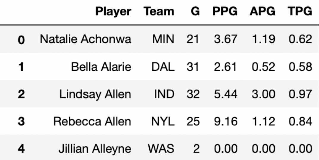
Each row in season corresponds to a single player. For
each player, we have: - 'Player' (str), their
name - 'Team' (str), the three-letter code of
the team they play on - 'G' (int), the number
of games they played in the 2021 season - 'PPG'
(float), the number of points they scored per game played -
'APG' (float), the number of assists (passes)
they made per game played - 'TPG' (float), the
number of turnovers they made per game played
Note that all of the numerical columns in season must
contain values that are greater than or equal to 0.
Which of the following is the best choice for the index of
season?
'Player'
'Team'
'G'
'PPG'
Answer: 'Player'
Ideally, the index of a DataFrame is unique, so that we can use it to
“identify” the rows. Here, each row is about a player, so
'Player' should be the index. 'Player' is the
only column that is likely to be unique; it is possible that two players
have the same name, but it’s still a better choice of index
than the other three options, which are definitely not unique.
The average score on this problem was 95%.
Note: For the rest of the exam, assume that the
index of season is still 0, 1, 2, 3, …
Below is a histogram showing the distribution of the number of
turnovers per game for all players in season.
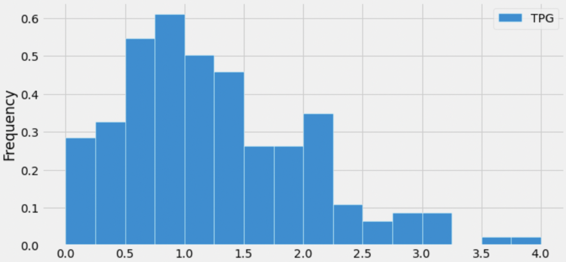
Suppose, throughout this question, that the mean number of turnovers per game is 1.25. Which of the following is closest to the median number of turnovers per game?
0.5
0.75
1
1.25
1.5
1.75
Answer: 1
The median of a distribution is the value that is “halfway” through the distribution, i.e. the value such that half of the values in the distribution are larger than it and half the values in the distribution are smaller than it.
Visually, we’re looking for the location on the x-axis where we can draw a vertical line that splits the area of the histogram in half. While it’s impossible to tell the exact median of the distribution, since we don’t know how the values are distributed within the bars, we can get pretty close by using this principle.
Immediately, we can rule out 0.5, 0.75, 1.5, and 1.75, since they are too far from the “center” of the distribution (imagine drawing vertical lines at any of those points on the x-axis; they don’t split the distribution’s area in half). To decide between 1 and 1.25, we can use the fact that the distribution is right-skewed, meaning that its mean is larger than its median (intuitively, the mean is dragged in the direction of the tail, which is to the right). This means that the median should be less than the mean. We are given that the mean of the distribution is 1.25, so the median should be 1.
The average score on this problem was 73%.
Sabrina Ionescu and Sami Whitcomb are both players on the New York Liberty, and are both California natives.
In “original units”, Sabrina Ionescu had 3.5 turnovers per game. In standard units, her turnovers per game is 3.
In standard units, Sami Whitcomb’s turnovers per game is -1. How many turnovers per game did Sami Whitcomb have in original units? Round your answer to 3 decimal places.
Note: You will need the fact from the previous subpart that the mean number of turnovers per game is 1.25.
Answer: 0.5
To convert a value x to standard units (denoted by x_{\text{su}}), we use the following formula:
x_{\text{su}} = \frac{x - \text{mean of }x}{\text{SD of }x}
Let’s look at the first line given to us: In “original units”, Sabrina Ionescu had 3.5 turnovers per game. In standard units, her turnovers per game is 3.
Substituting the information we know into the above equation gives us:
3 = \frac{3.5 - 1.25}{\text{SD of }x}
In order to convert future values from original units to standard units, we’ll need to know \text{SD of }x, which we don’t currently but can obtain by rearranging the above equation. Doing so yields
\text{SD of }x = \frac{3.5-1.25}{3} = \frac{2.25}{3} = 0.75
Now, let’s look at the second line we’re given: In standard units, Sami Whitcomb’s turnovers per game is -1. How many turnovers per game did Sami Whitcomb have in original units? Round your answer to 3 decimal places.
We have all the information we need to convert Sami Whitcomb’s turnovers per game from standard units to original units! Plugging in the values we know gives us:
\begin{aligned} x_{\text{su}} &= \frac{x - \text{mean of }x}{\text{SD of }x} \\ -1 &= \frac{x - 1.25}{0.75} \\ -0.75 &= x - 1.25 \\ 1.25 - 0.75 &= x \\ x &= \boxed{0.5} \end{aligned}
Thus, in original units, Sami Whitcomb averaged 0.5 turnovers per game.
The average score on this problem was 87%.
What is the smallest possible number of turnovers per game, in standard units? Round your answer to 3 decimal places.
Answer: -1.667
The smallest possible number of turnovers per game in original units is 0 (which a player would have if they never had a turnover – that would mean they’re really good!). To find the smallest possible turnovers per game in standard units, all we need to do is convert 0 from original units to standard units. This will involve our work from the previous subpart.
\begin{aligned} x_{\text{su}} &= \frac{x - \text{mean of }x}{\text{SD of }x} \\ &= \frac{0 - 1.25}{0.75} \\ &= -\frac{1.25}{0.75} \\ &= -\frac{5}{3} = \boxed{-1.667} \end{aligned}
The average score on this problem was 82%.
Recall that the mean points per game is 7, with a standard deviation of 5. Also note that for all players, points per game must be greater than or equal to 0.
Using Chebyshev’s inequality, we find that at least p\% of players scored 25 or fewer points per game.
What is the value of p? Give your answer as number between 0 and 100, rounded to 3 decimal places.
Answer: 92.284\%
Recall, Chebyshev’s inequality states that the proportion of values within z standard deviations of the mean is at least 1 - \frac{1}{z^2}.
To approach the problem, we’ll start by converting 25 points per game to standard units. Doing so yields \frac{25 - 7}{5} = 3.6. This means that 25 is 3.6 standard deviations above the mean. The value 3.6 standard deviations below the mean is 7 - 3.6 \cdot 5 = -11, so when we use Chebyshev’s inequality with z = 3.6, we will get a lower bound on the proportion of values between -11 and 25. However, as the question tells us, points per game must be non-negative, so in this case the proportion of values between -11 and 25 is the same as the proportion of values between 0 and 25 (i.e. the proportion of values less than or equal to 25).
When z = 3.6, we have 1 - \frac{1}{z^2} = 1 - \frac{1}{3.6^2} = 0.922839, which as a percentage rounded to three decimal places is 92.284\%. Thus, at least 92.284\% scored 25 or fewer points per game.
The average score on this problem was 46%.
Note: This problem is out of scope; it covers material no longer included in the course.
Note: This question uses the mathematical definition
of percentile, not np.percentile.
The array aces defined below contains the points per
game scored by all members of the Las Vegas Aces. Note that it contains
14 numbers that are in sorted order.
aces = np.array([0, 0, 1.05, 1.47, 1.96, 2, 3.25,
                 10.53, 11.09, 11.62, 12.19,
                 14.24, 14.81, 18.25])
As we saw in lab, percentiles are not unique. For instance, the
number 1.05 is both the 15th percentile and 16th percentile of
aces.
There is a positive integer q,
between 0 and 100, such that 14.24 is the qth percentile of aces, but
14.81 is the (q+1)th percentile of
aces.
What is the value of q? Give your answer as an integer between 0 and 100.
Answer: 85
For reference, recall that we find the pth percentile of a collection of n numbers as follows:
h = \frac{p}{100} \cdot n
If h is an integer, define k = h. Otherwise, let k be the smallest integer greater than h.
Take the kth element of the sorted collection (start counting from 1, not 0).
To start, it’s worth emphasizing that there are n = 14 numbers in aces total.
14.24 is at position 12 (when the positions are numbered 1 through
14).
Let’s try and find a value of p such that 14.24 is the pth percentile. To do so, we might try and find what “percentage” of the way through the distribution 14.24 is; doing so gives \frac{12}{14} = 85.71\%. If we follow the process outlined above with p = 85, we get that h = \frac{85}{100} \cdot 14 = 11.9 and thus k = 12, meaning that the 85th percentile is the number at position 12, which 14.24.
Let’s see what happens when we try the same process with p = 86. This time, we have h = \frac{86}{100} \cdot 14 = 12.04 and thus k = 13, meaning that the 86th percentile is the number at position 13, which is 14.81.
This means that the value of q is 85 – the 85th percentile is 14.24, while the 86th percentile is 14.81.
The average score on this problem was 57%.
Suppose that in Olympic ski jumping, ski jumpers jump off of a ramp that’s shaped like a portion of a normal curve. Drawn from left to right, a full normal curve has an inflection point on the ascent, then a peak, then another inflection point on the descent. A ski jump ramp stops at the point that is one third of the way between the inflection point on the ascent and the peak, measured horizontally. Below is an example ski jump ramp, along with the normal curve that generated it.
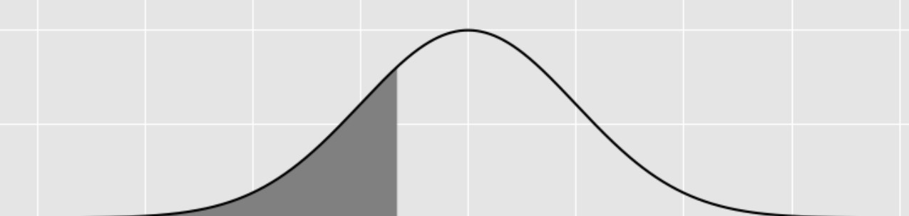
Fill in the blank below so that the expression evaluates to the area of a ski jump ramp, if the area under the normal curve that generated it is 1.
    from scipy import stats
    stats.norm.cdf(______)
What goes in the blank?
Answer: -2/3
We know that the normal distribution is symmetric about the mean, and
that the mean is the “peak” described in the graph. The inflection
points occur one standard deviation above and below the mean (the peak),
so a point which is one third of the way in between the first inflection
point and the peak is -(1-\frac{1}{3}) =
-\frac{2}{3} standard deviations from the mean. We can then use
stats.norm.cdf(-2/3) to calculate the area under the curve
to the left of this point.
The average score on this problem was 51%.
Suppose that in Olympic downhill skiing, skiers compete on mountains shaped like normal distributions with mean 50 and standard deviation 8. Skiers start at the peak and ski down the right side of the mountain, so their x-coordinate increases.
Keenan is an Olympic downhill skier, but he’s only been able to practice on a mountain shaped like a normal distribution with mean 65 and standard deviation 12. In his practice, Keenan always crouches down low when he reaches the point where his x-coordinate is 92, which helps him ski faster. When he competes at the Olympics, at what x-coordinate should he crouch down low, corresponding to the same relative location on the mountain?
Answer: 68
Since we know that both slopes are normal distributions (just scaled and shifted), we can derive this answer by writing Keenan’s crouch point in terms of standard deviations from the mean. He typically crouches at 92 feet, whose distance from the mean (in standard deviations) is given by \frac{92 - 65}{12} = 2.25. So, all we need to do is find what number is 2.25 standard deviations from the mean in the Olympic mountain. This is given by 50 + (2.25 * 8) = 68
The average score on this problem was 72%.
Aaron is another Olympic downhill skier. When he competes on the normal curve mountain with mean 50 and standard deviation 8, he crouches down low when his x-coordinate is 54. If the total area of the mountain is 1, approximately how much of the mountain’s area is ahead of Aaron at the moment he crouches down low?
0.1
0.2
0.3
0.4
Answer: 0.3
We know that when Aaron reaches the mean (50), exactly 0.5 of the mountain’s area is behind him, since the mean and median are equal for normal distributions like this one. We also see that 54 is one half of a standard deviation away from the mean. So, all we have to do is find out what proportion of the area is within half a standard deviation of the mean. Using the 68-95-99.7 rule, we know that 68% of the values lie within one standard deviation of the mean to both the right and left side. So, this means 34% of the values are within one standard deviation on one side and at least 17% are within half a standard deviation on one side. Since the area is 1, the area would be 0.17. So, by the time Aaron reaches an x-coordinate of 54, 0.5 + 0.17 = 0.67 of the mountain is behind him. From here, we simply calculate the area in front by 1 - 0.67 = 0.33, so we conclude that approximately 0.3 of the area is in front of Aaron.
Note: As a clafrification, the 0.17 is an estimate, specifically, an underestimate, due to the shape of the normal distribution. Thse area under a normal distribution is not proportional to how many standard deviations far away from the mean you are.
The average score on this problem was 50%.
Suppose we’ve imported the scipy module. To the nearest
0.5, what does the following expression evaluate to?
scipy.stats.norm.cdf(-2) * 100
Answer: 2.5
The average score on this problem was 57%.
Beneath Gringotts Wizarding Bank, enchanted mine carts transport wizards through a complex underground railway on the way to their bank vault.
During one section of the journey to Harry’s vault, the track follows the shape of a normal curve, with a peak at x = 50 and a standard deviation of 20.
A ferocious dragon, who lives under this section of the railway, is equally likely to be located anywhere within this region. What is the probability that the dragon is located in a position with x \leq 10 or x \geq 80? Select all that apply.
1 - (scipy.stats.norm.cdf(1.5) - scipy.stats.norm.cdf(-2))
2 * scipy.stats.norm.cdf(1.75)
scipy.stats.norm.cdf(-2) + scipy.stats.norm.cdf(-1.5)
0.95
None of the above.
Answer:
1 - (scipy.stats.norm.cdf(1.5) - scipy.stats.norm.cdf(-2))
&
scipy.stats.norm.cdf(-2) + scipy.stats.norm.cdf(-1.5)
Option 1: This code calculates the probability that a value lies outside the range between z = -2 and z = 1.5, which corresponds to x \leq 10 or x \geq 80. This is done by subtracting the area under the normal curve between -2 and 1.5 from 1. This is correct because it accurately captures the combined probability in the left and right tails of the distribution.
Option 2: This code multiplies the cumulative distribution function (CDF) at z = 1.75 by 2. This assumes symmetry around the mean and is used for intervals like |z| \geq 1.75, but that’s not what we want. The correct z-values for this problem are -2 and 1.5, so this option is incorrect.
Option 3: This code adds the probability of z \leq -2 and z \geq 1.5, using the fact that P(z \geq 1.5) = P(z \leq -1.5) by symmetry. So, while the code appears to show both as left-tail calculations, it actually produces the correct total tail probability. This option is correct.
Option 4: This is a static value with no basis in the z-scores of -2 and 1.5. It’s likely meant as a distractor and does not represent the correct probability for the specified conditions. This option is incorrect.
Harry wants to know where, in this section of the track, the cart’s height is changing the fastest. He knows from his earlier public school education that the height changes the fastest at the inflection points of a normal distribution. Where are the inflection points in this section of the track?
x = 50
x = 20 and x = 80
x = 30 and x = 70
x = 0 and x = 100
Answer: x = 30 and x = 70
Recall that the inflection points of a normal distribution are located one standard deviation away from the mean. In this problem, the mean is x = 50 and the standard deviation is 20, so the inflection points occur at x = 30 and x = 70. These are the points where the curve changes concavity and where the height is changing the fastest. Therefore, the correct answer is x = 30 and x = 70.
Next, consider a different region of the track, where the shape follows some arbitrary distribution with mean 130 and standard deviation 30. We don’t have any information about the shape of the distribution, so it is not necessarily normal.
What is the minimum proportion of area under this section of the track within the range 100 \leq x \leq 190?
0.77
0.55
0.38
0.00
Answer: 0.00
We are told that the distribution is not necessarily normal. The mean is 130 and the standard deviation is 30. We’re asked for the minimum proportion of area between x = 100 and x = 190.
Since the distribution isn’t normal and we don’t know its shape, we can’t use the empirical rule (68-95-99.7) or z-scores. We might try using Chebyshev’s Inequality, but that only works for intervals that are equally far below the mean as above the mean. This interval is not like that (it’s 1 standard deviation below the mean and 2 above), so Chebyshev’s Inequality doesn’t apply. The most we can say using Chebyshev’s Inequality is that in the interval from 1 standard deviation below the mean to 1 standard deviation above the mean, we can get at least 1 - \frac{1}{0^2} = 0 percent of the data. We can’t make any additional guarantees. So, the minimum possible proportion of area is 0.00.
Your friend at SDSU records the number of students who visit their library each day, for 100 days. They tell you that the average is 6{,}000 and that the standard deviation is 500.
Without knowing anything about the distribution of your friend’s data, find the endpoints of the smallest interval which is guaranteed to contain at least 75\% of your friend’s data. Both endpoints should be given as integers.
Answer: [5000, 7000]
The average score on this problem was 64%.
If you then learn that your friend’s data is normally distributed, approximately what percentage of the data is actually contained in the interval you found above? Give your answer as an integer.
Answer: 95\%
The average score on this problem was 75%.
Minchan wants to see his listening trends. Suppose he takes many
samples of size 30 from plays_minchan and computes their
means. For each statement below, select the best answer.
(a) We expect that at least 75% of all of the
sampled values of plays_minchan lie within 2 standard
deviations of the population mean.
Yes, due to CLT
Yes, due to Chebyshev’s
No, due to CLT
No, due to Chebyshev’s
Yes, but for reasons that have nothing to do with Chebyshev’s or the CLT
No, but for reasons that have nothing to do with Chebyshev’s or the CLT
Answer: Yes, due to Chebyshev’s
This statement is about individual data values, not sample means. Chebyshev’s inequality guarantees that at least 1 - 1/k^2 of data lies within k standard deviations of the mean. With k=2, that’s at least 1 - 1/4 = 75\%.
The average score on this problem was 78%.
(b) We expect that approximately 95% of all sample means lie within 2 standard errors of the population mean.
Yes, due to CLT
Yes, due to Chebyshev’s
No, due to CLT
No, due to Chebyshev’s
Yes, but for reasons that have nothing to do with Chebyshev’s or the CLT
No, but for reasons that have nothing to do with Chebyshev’s or the CLT
Answer: Yes, due to CLT
With a sample size of 30, the CLT tells us the distribution of sample means is approximately normal. For a normal distribution, approximately 95% of values lie within 2 standard deviations (standard errors) of the mean.
The average score on this problem was 66%.
(c) Now assume the distribution of
plays_minchan is right-skewed but with no outliers. Which
of the following statements is true about these statistics of
plays_minchan?
The median is always greater than the mean
The mean is always greater than the median
The mean is usually greater than the median, but not always
The median is usually greater than the mean, but not always
Answer: The mean is usually greater than the median, but not always
In a right-skewed distribution, the long tail on the right pulls the mean upward, so the mean is typically greater than the median. However, this is not a strict rule — it’s possible to construct right-skewed distributions where the mean is less than the median.
The average score on this problem was 45%.
(d) If both Minchan’s and Ray’s plays distributions are normal, will the distribution formed by pooling both of their plays into one combined dataset be approximately normal?
Always
Sometimes
Never
Answer: Sometimes
A mixture of two normal distributions is not necessarily normal. If the two distributions have very different means, the combined distribution may be bimodal. However, if the means and standard deviations are similar enough, the result could still appear approximately normal.
The average score on this problem was 49%.
(a) Ray calculated a 95% CLT-based confidence interval for the population mean of his number of plays per song, spanning [60.5, 100.5]. If the sample size used to construct the interval was 25 songs, what is the standard deviation of Ray’s plays?
Note: “Not enough information” is also a possible answer.
Answer: 50
The width of the interval is 100.5 - 60.5 = 40, so the half-width is 20. For a 95% CI, half-width = 2 \times \frac{SD}{\sqrt{n}}. With n = 25: 20 = 2 \times \frac{SD}{5}, so SD = 50.
The average score on this problem was 24%.
(b) If Ray increases the sample size from 25 songs to 100 songs, how does the width of his 95% CLT-based confidence interval change?
Doubles
Halves
Becomes 1/4 as wide
Stays the same
Answer: Halves
The width of a CI is proportional to \frac{1}{\sqrt{n}}. Going from n=25 to n=100 multiplies the sample size by 4, so the width is multiplied by \frac{1}{\sqrt{4}} = \frac{1}{2}, i.e., it halves.
The average score on this problem was 63%.
(c) Now Ray is curious about other confidence
intervals he could have constructed. Given
stats.norm.cdf(1.75) = 0.96, calculate the endpoints of a
92% CLT-based confidence interval.
Note: “Not enough information” is also a possible answer.
Answer: [63, 98]
For a 92% CI, we need 4% in each tail. Since
stats.norm.cdf(1.75) = 0.96, the z-score is 1.75. The
sample mean is the midpoint: (60.5 + 100.5)/2
= 80.5. The SE = SD/\sqrt{n} = 50/5 =
10. The 92% CI is 80.5 \pm 1.75 \times
10 = 80.5 \pm 17.5, giving [63,
98].
The average score on this problem was 63%.
(d) Ray then constructs a 99% CLT-based confidence interval. Select all the cases that could be possible when comparing his new 99% CI to his original 95% CI.
99% CI is wider than 95%
99% CI is smaller than 95%
They have the same width
Answer: 99% CI is wider than 95%
A higher confidence level requires a larger z-score, which always produces a wider interval (given the same sample). So the 99% CI is always wider than the 95% CI.
The average score on this problem was 84%.