← return to practice.dsc10.com
Below are practice problems tagged for Lecture 17 (rendered directly from the original exam/quiz sources).
The Museum of Natural History has a large collection of dinosaur bones, and they know the approximate year each bone is from. They want to use this sample of dinosaur bones to estimate the total number of years that dinosaurs lived on Earth. We’ll make the assumption that the sample is a uniform random sample from the population of all dinosaur bones. Which statistic below will give the best estimate of the population parameter?
sample sum
sample max - sample min
2 \cdot (sample mean - sample min)
2 \cdot (sample max - sample mean)
2 \cdot sample mean
2 \cdot sample median
Answer: sample max - sample min
Our goal is to estimate the total number of years that dinosaurs lived on Earth. In other words, we want to know the range of time that dinosaurs lived on Earth, and by definition range = biggest value - smallest value. By using “sample max - sample min”, we calculate the difference between the earliest and the latest dinosaur bones in this uniform random sample, which helps us to estimate the population range.
The average score on this problem was 52%.
The curator at the Museum of Natural History, who happens to have taken a data science course in college, points out that the estimate of the parameter obtained from this sample could certainly have come out differently, if the museum had started with a different sample of bones. The curator suggests trying to understand the distribution of the sample statistic. Which of the following would be an appropriate way to create that distribution?
bootstrapping the original sample
using the Central Limit Theorem
both bootstrapping and the Central Limit Theorem
neither bootstrapping nor the Central Limit Theorem
Answer: neither bootstrapping nor the Central Limit Theorem
Recall, the Central Limit Theorem (CLT) says that the probability distribution of the sum or average of a large random sample drawn with replacement will be roughly normal, regardless of the distribution of the population from which the sample is drawn. Thus, the theorem only applies when our sample statistics is sum or average, while in this question, our statistics is range, so CLT does not apply.
Bootstrapping is a valid technique for estimating measures of central tendency, e.g. the population mean, median, standard deviation, etc. It doesn’t work well in estimating extreme or sensitive values, like the population maximum or minimum. Since the statistic we’re trying to estimate is the difference between the population maximum and population minimum, bootstrapping is not appropriate.
The average score on this problem was 20%.
The credit card company that owns the data in apps,
BruinCard, has decided not to give us access to the entire
apps DataFrame, but instead just a random sample of 100
rows of apps called hundred_apps.
We are interested in estimating the mean age of all applicants in
apps given only the data in hundred_apps. The
ages in hundred_apps have a mean of 35 and a standard
deviation of 10.
Give the endpoints of the CLT-based 95% confidence interval for the
mean age of all applicants in apps, based on the data in
hundred_apps.
Answer: Left endpoint = 33, Right endpoint = 37
According to the Central Limit Theorem, the standard deviation of the distribution of the sample mean is \frac{\text{sample SD}}{\sqrt{\text{sample size}}} = \frac{10}{\sqrt{100}} = 1. Then using the fact that the distribution of the sample mean is roughly normal, since 95% of the area of a normal curve falls within two standard deviations of the mean, we can find the endpoints of the 95% CLT-based confidence interval as 35 - 2 = 33 and 35 + 2 = 37.
We can think of this as using the formula below: \left[\text{sample mean} - 2\cdot \frac{\text{sample SD}}{\sqrt{\text{sample size}}}, \: \text{sample mean} + 2\cdot \frac{\text{sample SD}}{\sqrt{\text{sample size}}} \right]. Plugging in the appropriate quantities yields [35 - 2\cdot\frac{10}{\sqrt{100}}, 35 - 2\cdot\frac{10}{\sqrt{100}}] = [33, 37].
The average score on this problem was 67%.
BruinCard reinstates our access to apps so that we can
now easily extract information about the ages of all applicants. We
determine that, just like in hundred_apps, the ages in
apps have a mean of 35 and a standard deviation of 10. This
raises the question of how other samples of 100 rows of
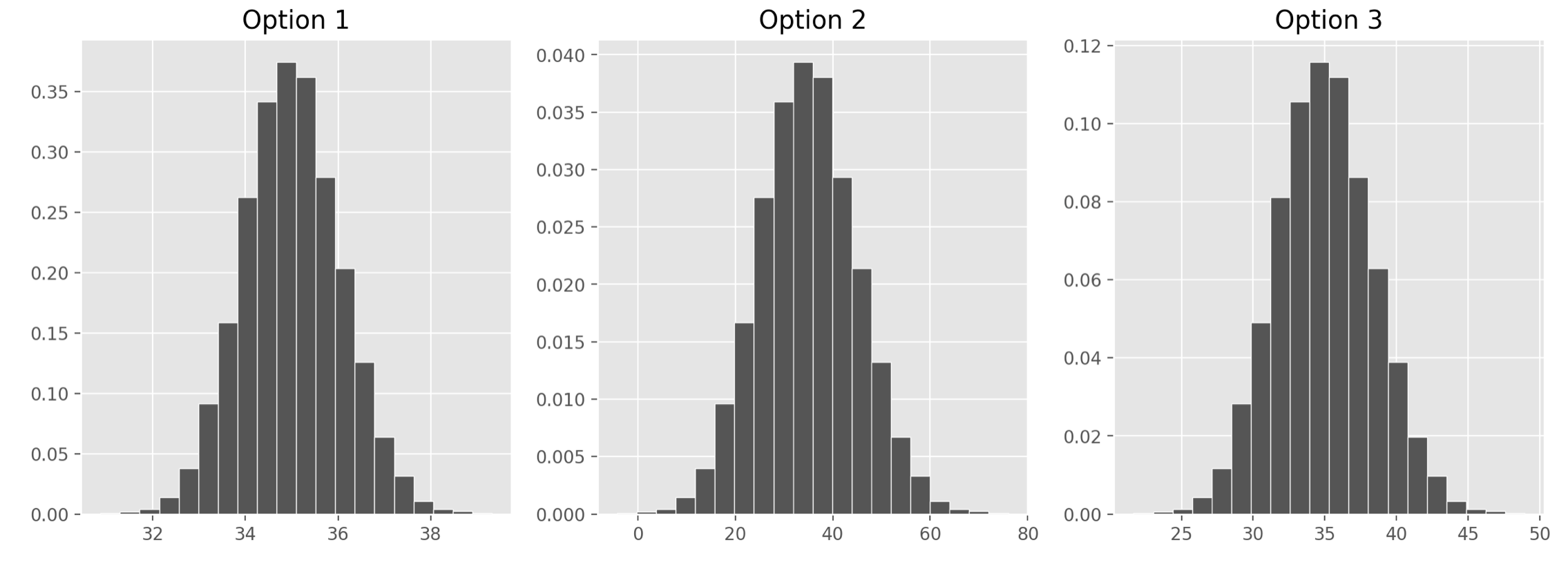
apps would have turned out, so we compute 10,000 sample means as follows.
    sample_means = np.array([])
    for i in np.arange(10000):
        sample_mean = apps.sample(100, replace=True).get("age").mean()
sample_means = np.append(sample_means, sample_mean)Which of the following three visualizations best depict the
distribution of sample_means?
Answer: Option 1
As we found in the previous part, the distribution of the sample mean should have a standard deviation of 1. We also know it should be centered at the mean of our sample, at 35, but since all the options are centered here, that’s not too helpful. Only Option 1, however, has a standard deviation of 1. Remember, we can approximate the standard deviation of a normal curve as the distance between the mean and either of the inflection points. Only Option 1 looks like it has inflection points at 34 and 36, a distance of 1 from the mean of 35.
If you chose Option 2, you probably confused the standard deviation of our original sample, 10, with the standard deviation of the distribution of the sample mean, which comes from dividing that value by the square root of the sample size.
The average score on this problem was 57%.
Which of the following statements are guaranteed to be true? Select all that apply.
We used bootstrapping to compute sample_means.
The ages of credit card applicants are roughly normally distributed.
A CLT-based 90% confidence interval for the mean age of credit card applicants, based on the data in hundred apps, would be narrower than the interval you gave in part (a).
The expression np.percentile(sample_means, 2.5)
evaluates to the left endpoint of the interval you gave in part (a).
If we used the data in hundred_apps to create 1,000
CLT-based 95% confidence intervals for the mean age of applicants in
apps, approximately 950 of them would contain the true mean
age of applicants in apps.
None of the above.
Answer: A CLT-based 90% confidence interval for the
mean age of credit card applicants, based on the data in
hundred_apps, would be narrower than the interval you gave
in part (a).
Let’s analyze each of the options:
Option 1: We are not using bootstrapping to compute sample means
since we are sampling from the apps DataFrame, which is our
population here. If we were bootstrapping, we’d need to sample from our
first sample, which is hundred_apps.
Option 2: We can’t be sure what the distribution of the ages of
credit card applicants are. The Central Limit Theorem says that the
distribution of sample_means is roughly normally
distributed, but we know nothing about the population
distribution.
Option 3: The CLT-based 95% confidence interval that we calculated in part (a) was computed as follows: \left[\text{sample mean} - 2\cdot \frac{\text{sample SD}}{\sqrt{\text{sample size}}}, \text{sample mean} + 2\cdot \frac{\text{sample SD}}{\sqrt{\text{sample size}}} \right] A CLT-based 90% confidence interval would be computed as \left[\text{sample mean} - z\cdot \frac{\text{sample SD}}{\sqrt{\text{sample size}}}, \text{sample mean} + z\cdot \frac{\text{sample SD}}{\sqrt{\text{sample size}}} \right] for some value of z less than 2. We know that 95% of the area of a normal curve is within two standard deviations of the mean, so to only pick up 90% of the area, we’d have to go slightly less than 2 standard deviations away. This means the 90% confidence interval will be narrower than the 95% confidence interval.
Option 4: The left endpoint of the interval from part (a) was
calculated using the Central Limit Theorem, whereas using
np.percentile(sample_means, 2.5) is calculated empirically,
using the data in sample_means. Empirically calculating a
confidence interval doesn’t necessarily always give the exact same
endpoints as using the Central Limit Theorem, but it should give you
values close to those endpoints. These values are likely very similar
but they are not guaranteed to be the same. One way to see this is that
if we ran the code to generate sample_means again, we’d
probably get a different value for
np.percentile(sample_means, 2.5).
Option 5: The key observation is that if we used the data in
hundred_apps to create 1,000 CLT-based 95% confidence
intervals for the mean age of applicants in apps, all of
these intervals would be exactly the same. Given a sample, there is only
one CLT-based 95% confidence interval associated with it. In our case,
given the sample hundred_apps, the one and only CLT-based
95% confidence interval based on this sample is the one we found in part
(a). Therefore if we generated 1,000 of these intervals, either they
would all contain the parameter or none of them would. In order for a
statement like the one here to be true, we would need to collect 1,000
different samples, and calculate a confidence interval from each
one.
The average score on this problem was 49%.
Among all Costco members in San Diego, the average monthly spending in October 2023 was $350 with a standard deviation of $40.
The amount Ciro spent at Costco in October 2023 was -1.5 in standard units. What is this amount in dollars? Give your answer as an integer.
Answer: 290
The average score on this problem was 93%.
What is the minimum possible percentage of San Diego members that spent between $250 and $450 in October 2023?
16%
22%
36%
60%
78%
84%
Answer: 84%
The average score on this problem was 61%.
Now, suppose we’re given that the distribution of monthly spending in October 2023 for all San Diego members is roughly normal. Given this fact, fill in the blanks:
What are m and n? Give your answers as integers rounded to the nearest multiple of 10.
Answer: m: 270, n: 430
The average score on this problem was 81%.
Matilda has been working at Bill’s Book Bonanza since it first opened
and her shifts for each week are always randomly scheduled (i.e., she
does not work the same shifts each week). Due to the system restrictions
at the bookstore, when Matilda logs in with her employee ID, she only
has access to the history of sales made during her shifts. Suppose these
transactions are stored in a DataFrame called matilda,
which has the same columns as the sales DataFrame that
stores all transactions.
Matilda wants to use her random sample to estimate the mean
price of books purchased with cash at Bill’s Book Bonanza. For
the purposes of this question, assume Matilda only has access to
matilda, and not all of sales.
Complete the code below so that cash_left and
cash_right store the endpoints of an 86\% bootstrapped confidence interval for the
mean price of books purchased with cash at Bill’s Book Bonanza.
    cash_means = np.array([])
    original = __(a)__
    for i in np.arange(10000):
        resample = original.sample(__(b)__)
        cash_means = np.append(cash_means, __(c)__)

    cash_left = __(d)__
cash_right = __(e)__matilda[matilda.get("cash")]We first filter the matilda DataFrame to only include
rows where the payment method was cash, since these are the only rows
that are relevant to our question of the mean price of books purchased
with cash.
The average score on this problem was 65%.
original.shape[0], replace = TrueWe repeatedly resample from this filtered data. We always bootstrap using the same sample size as the original sample, and with replacement.
The average score on this problem was 79%.
resample.get("price").mean()Our statistic is the mean price, which we need to calculate from the
resample DataFrame.
The average score on this problem was 71%.
np.percentile(cash_means, 7)Since our goal is to construct an 86% confidence interval, we take the 7^{th} percentile as the left endpoint and the 93^{rd} percentile as the right endpoint. These numbers come from 100 - 86 = 14, which means we want 14\% of the area excluded from our interval, and we want to split that up evenly with 7\% on each side.
The average score on this problem was 84%.
np.percentile(cash_means, 93)
The average score on this problem was 84%.
Next, Matilda uses the data in matilda to construct a
95\% CLT-based confidence interval for
the same parameter.
Given that there are 400 cash transactions in matilda
and her confidence interval comes out as [19.58, 21.58], what is the standard
deviation of the prices of all cash transactions at Bill’s Book
Bonanza?
Answer: 10
The width of the interval is 21.58 - 19.58 = 2. Using the formula for the width of a 95\% CLT-based confidence interval and solving for the standard deviation gives the answer.
Width = 4 * \frac{SD}{\sqrt{400}}
SD = 2 * \frac{\sqrt{400}}{4} = 10
The average score on this problem was 61%.
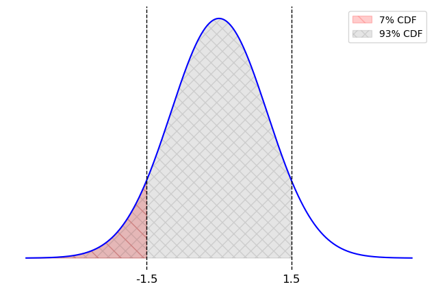
Knowing the endpoints of Matilda’s 95% CLT-based confidence interval can actually help us to determine the endpoints of her 86% bootstrapped confidence interval. You may also need to know the following facts:
stats.norm.cdf(1.1) evaluates to
0.86
stats.norm.cdf(1.5) evaluates to
0.93
Estimate the value of cash_left to one decimal
place.
Answer: 19.8
The useful fact here is the second fact. It says that if you step 1.5 standard deviations to the right of the mean in a normal distribution, 93% of the area will be to the left. Since that leaves 7% of the area to the right, this also means that the area to the left of -1.5 standard units is 7%, by symmetry. So the area between -1.5 and 1.5 standard units is 86% of the area, or the bounds for an 86% confidence interval. This is the grey area in the picture below.
The middle of our interval is 20.58 so we calculate the left endpoint as:
\begin{align*} \texttt{cash\_left} &= 20.58 - 1.5 * \frac{SD}{\sqrt{n}}\\ &= 20.58 - 1.5 * \frac{10}{\sqrt{400}}\\ &= 20.58 - 0.75 \\ &= 19.83\\ &\approx 19.8 \end{align*}
The average score on this problem was 22%.
Which of the following are valid conclusions? Select all that apply.
Approximately 95% of the values in cash_means fall
within the interval [19.58, 21.58].
Approximately 95% of books purchased with cash at Bill’s Book Bonanza have a price that falls within the interval [19.58, 21.58].
The actual mean price of books purchased with cash at Bill’s Book Bonanza has a 95% chance of falling within the interval [19.58, 21.58].
None of the above.
Answer: Approximately 95% of the values in
cash_means fall within the interval [19.58, 21.58].
Choice 1 is correct because of the way bootstrapped confidence
intervals are created. If we made a 95% bootstrapped confidence interval
from cash_means, it would capture 95% of the values in cash_means,
by design. This is not how the interval [19.58, 21.58] was created, however; this
interval comes from the CLT. However bootstrapped and CLT-based
confidence intervals give very nearly the same results. They are two
methods to solve the same problem and they create nearly identical
confidence intervals. So it is correct to say that approximately 95% of
the values in cash_means fall within a 95% CLT-based
confidence interval, which is [19.58,
21.58].
Choice 2 is incorrect because the interval estimates the mean price, not individual book prices.
Choice 3 is incorrect because confidence intervals are about the reliability of the method: if we repeated the whole bootstrapping process many times, about 95% of the intervals would contain the true mean. It does not indicate the probability of the true mean being within this specific interval because this interval is fixed and the true mean is also fixed. It doesn’t make sense to talk about the probability of a fixed number falling in a fixed interval; that’s like asking if there’s a 95% chance that 5 is between 2 and 10.
The average score on this problem was 63%.
Matilda has been wondering whether the mean price of books purchased with cash at Bill’s Book Bonanza is \$20. What can she conclude about this?
The mean price of books purchased with cash at Bill’s Book Bonanza is $20.
The mean price of books purchased with cash at Bill’s Book Bonanza could plausibly be $20.
The mean price of books purchased with cash at Bill’s Book Bonanza is not $20.
The mean price of books purchased with cash at Bill’s Book Bonanza is most likely not $20.
Answer: The mean price of books purchased with cash at Bill’s Book Bonanza could plausibly be $20.
This question is referring to a hypothesis test where we test whether parameter (in this case, the mean price of books purchased with cash) is equal to a specific value ($20). The hypothesis test can be conducted by constructing a confidence interval for the parameter and checking whether the specific value falls in the interval. Since $20 is within the confidence interval, it is a plausible value for the parameter, but never guaranteed.
The average score on this problem was 90%.
As in the previous problem, suppose we are told that
sales contains 1000 rows, 500 of which represent cash
transactions and 500 of which represent non-cash transactions.
This time, instead of being given histograms, we are told that the
distribution of "price" for cash transactions is roughly
normal, with a mean of \$14 and a
standard deviation of \$2. We’ll call
this distribution the cash curve.
Additionally, the distribution of "price" for non-cash
transactions is roughly normal, with a mean of \$22 and a standard deviation of \$4. We’ll call this distribution the
non-cash curve.
We want to draw a curve representing the approximate distribution of
"price" for all transactions combined. We’ll call this
distribution the combined curve.
What is the approximate proportion of area under the cash curve between \$10 and \$12? Your answer should be a number between 0 and 1.
Answer: 0.135
We know that for a normal distribution, approximately
For the cash curve, the mean is $14 and the standard deviation is $2, so using this rule:
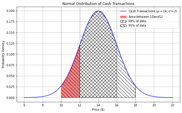
Area from $10 to $12 = Area from $10 to $14 - Area from $12 to $14 = 47.5% - 34% = 13.5% = 0.135
The average score on this problem was 46%.
Fill in the blanks in the code below so that the expression evaluates to the approximate proportion of area under the cash curve between \$14.50 and \$17.50. Each answer should be a single number.
scipy.stats.norm.cdf(a) - scipy.stats.norm.cdf(b)(a). Answer: 1.75
(b). Answer: 0.25
The expression
scipy.stats.norm.cdf(a) - scipy.stats.norm.cdf(b)
calculates the area under the normal distribution curve between two
points, where a is the right endpoint and b is
the left endpoint. Here, we’ll let a and b
represent the standardized values corresponding to $17.50 and $14.50,
respectively.
We’ll use the formula for standard units:
x_{i \: \text{(su)}} = \frac{x_i - \text{mean of $x$}}{\text{SD of $x$}}
For the standard units value corresponding to $17.50:
a = \frac{(17.50 - 14)}{2} = 1.75
For the standard units value corresponding to $14.50:
b = \frac{(14.50 - 14)}{2} = 0.25
The average score on this problem was 54%.
Will the combined curve be roughly normal?
Yes, because of the Central Limit Theorem.
Yes, because combining two normal distributions always produces a normal distribution.
No, not necessarily.
Answer: No, not necessarily.
Although both distributions are roughly normal, their means are significantly apart - one centered at 14 (with a standard deviation of 2) and one centered at 22 (with a standard deviation of 4). The resulting distribution is likely bimodal (having two peaks). The combined distribution will have peaks near each of the original means, reflecting the characteristics of the two separate normal distributions.
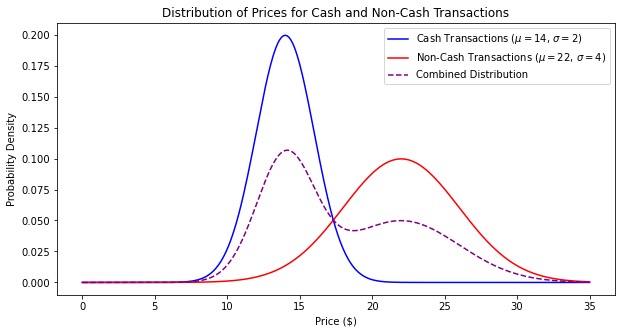
The CLT says that “the distribution of possible sample means is approximately normal, no matter the distribution of the population,” but it doesn’t say anything about combining two distributions.
The average score on this problem was 38%.
Fill in the blanks in the code below so that the expression evaluates to the approximate proportion of area under the combined curve between \$14 and \$22. Each answer should be a single number.
(scipy.stats.norm.cdf(a) - scipy.stats.norm.cdf(b)) / 2(a). Answer: 4
(b). Answer: -2
Since the the combined curve is a combination of two normal distributions, each representing equal number of transactions (500 each), we can approximate the total area by averaging the areas under the individual cash and non-cash curves between \$14 and \$22.
For cash:
P(Z ≤ \frac{22-14}{2}) - P(Z ≤ \frac{14-14}{2})
P(Z ≤ 4) - P(Z ≤ 0) = scipy.stats.norm.cdf(4) - scipy.stats.norm.cdf(0)
Non-cash:
P(Z ≤ \frac{22-22}{4}) - P(Z ≤ \frac{14-22}{4})
P(Z ≤ 0) - P(Z ≤ -2) = scipy.stats.norm.cdf(0) - scipy.stats.norm.cdf(-2)
Averaging area under the two distributions:
\frac{1}{2} (scipy.stats.norm.cdf(4) - scipy.stats.norm.cdf(0) + scipy.stats.norm.cdf(0) - scipy.stats.norm.cdf(-2)) = (scipy.stats.norm.cdf(4) - scipy.stats.norm.cdf(-2)) / 2
The average score on this problem was 15%.
What is the approximate proportion of area under the combined curve between \$14 and \$22? Choose the closest answer below.
0.47
0.49
0.5
0.95
0.97
Answer: 0.49
We can approximate the total area by averaging the areas under the individual cash and non-cash curves between \$14 and \$22.
Averaging the two individual areas: \frac{0.5 + 0.475}{2} = 0.4875, which is closest to 0.49.
The average score on this problem was 24%.
Statistica’s forests are filled with tall creatures called whingdingdillies. You have a large random sample of 400 whingdingdillies. In this sample, the mean height is 30m and the standard deviation is 4m. Suppose that whingdingdilly heights are normally distributed.
What are the endpoints of a CLT-based 95% confidence interval for the mean height of whingdingdillies? Each value should be a single number.
Answer: left endpoint = 29.6, right endpoint = 30.4
The average score on this problem was 50%.
Determine the values of the variables v and
w in the code below so that wdd_prop evaluates
to the approximate proportion of whingdingdillies with heights between
30m and 33m. Each value should be a single number.
wdd_prop = stats.norm.cdf(v) - stats.norm.cdf(w)Answer: v = .75, w = 0
The average score on this problem was 52%.
Above, we stated an assumption that whingdingdilly heights are normally distributed. For which part(s) of this question did we need that assumption?
2.1 only
2.2 only
both 2.1 and 2.2
neither 2.1 nor 2.2
Answer: 2.2 only
The average score on this problem was 57%.
After a frightening encounter, you discover that whingdingdillies can run very fast. You collect a sample of 400 whingdingdilly speeds, then use this sample to generate a bootstrapped distribution of resample mean speeds. Afterwards, you wonder how your bootstrapped distribution would have looked if you had instead been able to collect a random sample of size 900. Which of the following overlaid histograms shows two bootstrapped distributions of resample mean speeds, based on samples of size 400 and 900?

Answer: Option A
The average score on this problem was 59%.
Ryan writes the following code to obtain a 95% bootstrapped confidence interval for the mean number of students in Geisel’s second floor at 10AM in the fall only:
stats = np.array([])
for i in range(3333):
    stat = fall.sample(fall.shape[0],
                       replace=True).get("students").mean()
    stats = np.append(stats, stat)
lower = np.percentile(stats, 2.5)
upper = np.percentile(stats, 97.5)Write one line of code that evaluates to the upper endpoint of the 95\% CLT-based confidence interval for this same parameter. Recall that some potentially relevant values are provided with the DataFrames on the previous page.
Answer:
400 + 2 * 10 / fall.shape[0] ** 0.5
The average score on this problem was 65%.
True or False: The 95\% confidence interval generated by the bootstrapping code above cannot be narrower than a 95% confidence interval generated by the Central Limit Theorem.
True
False
Answer: False
The average score on this problem was 69%.
True or False: The Central Limit Theorem tells us
that the data in fall.get("students") is roughly normally
distributed.
True
False
Answer: False
The average score on this problem was 62%.
True or False: To obtain a 95% bootstrapped
confidence interval for the median, we can simply change
.mean() to .median() in the original code
above.
True
False
Answer: True
The average score on this problem was 80%.
True or False: We can use the CLT to create a valid 95\% confidence interval for the median.
True
False
Answer: False
The average score on this problem was 86%.
An IKEA employee has access to a data set of the purchase amounts for 40,000 customer transactions. This data set is roughly normally distributed with mean 150 dollars and standard deviation 25 dollars.
Why is the distribution of purchase amounts roughly normal?
because of the Central Limit Theorem
for some other reason
Answer: for some other reason
The data that we have is a sample of purchase amounts. It is not a sample mean or sample sum, so the Central Limit Theorem does not apply. The data just naturally happens to be roughly normally distributed, like human heights, for example.
The average score on this problem was 42%.
Shiv spends 300 dollars at IKEA. How would we describe Shiv’s purchase in standard units?
0 standard units
2 standard units
4 standard units
6 standard units
Answer: 6 standard units
To standardize a data value, we subtract the mean of the distribution and divide by the standard deviation:
\begin{aligned} \text{standard units} &= \frac{300 - 150}{25} \\ &= \frac{150}{25} \\ &= 6 \end{aligned}
A more intuitive way to think about standard units is the number of standard deviations above the mean (where negative means below the mean). Here, Shiv spent 150 dollars more than average. One standard deviation is 25 dollars, so 150 dollars is six standard deviations.
The average score on this problem was 97%.
Give the endpoints of the CLT-based 95% confidence interval for the mean IKEA purchase amount, based on this data.
Answer: 149.75 and 150.25 dollars
The Central Limit Theorem tells us about the distribution of the sample mean purchase amount. That’s not the distribution the employee has, but rather a distribution that shows how the mean of a different sample of 40,000 purchases might have turned out. Specifically, we know the following information about the distribution of the sample mean.
Since the distribution of the sample mean is roughly normal, we can find a 95% confidence interval for the sample mean by stepping out two standard deviations from the center, using the fact that 95% of the area of a normal distribution falls within 2 standard deviations of the mean. Therefore the endpoints of the CLT-based 95% confidence interval for the mean IKEA purchase amount are
The average score on this problem was 36%.
Which of the following quantities must be known in order to construct a CLT-based confidence interval for the population mean? Select all that apply.
Shape of the population (normal or not)
Shape of the sample (normal or not)
Mean of the population
Mean of the sample
Standard deviation of the population
Standard deviation of the sample
Size of the population
Size of the sample
Answer: Mean of the sample, Standard deviation of the sample, Size of the sample
The average score on this problem was 73%.
After this year’s Sun God Festival, the UCSD administration wants to estimate how much students would be willing to pay for a ticket to future Sun God Festivals. They (somehow) take 500 simple random samples of 100 students each, asking them this question. They then plot a histogram showing the distribution of the mean response from each sample.
Which of the following statements are true? Select all that apply.
The histogram will be approximately centered around the mean amount that all UCSD students would be willing to pay.
The variability in the histogram is due to the fact that we resample with replacement.
This distribution is an example of an empirical distribution.
This distribution includes many randomly generated parameters.
None of the above.
Answer: Options 1 and 3
The average score on this problem was 88%.
Describe in one word how the histogram would be different if it were instead based on 500 simple random samples of 1000 students each.
Answer: narrower
The average score on this problem was 70%.
According to Indeed, a popular job website, the hourly pay for data science interns across the US has a mean of 24 and a standard deviation of 6. You take a random sample of 64 data science interns. In your sample, the hourly pay has a mean of 25 and a standard deviation of 4. Suppose you bootstrap your sample 10,000 times, calculate the mean hourly pay from each resample, and plot a histogram of these resampled means. Which of the following best describes this histogram?
Roughly normal with a mean of 24 and a standard deviation of 6.
Roughly normal with a mean of 24 and a standard deviation of 0.75.
Roughly normal with a mean of 25 and a standard deviation of 4.
Roughly normal with a mean of 25 and a standard deviation of 0.5.
None of the above.
Answer: Option 4
The average score on this problem was 50%.
You are interested in estimating the average wait time between an interview and an internship offer being made. You take a random sample of n internship offers and find that in this sample, the average wait time is d days and the standard deviation is 4 days.
You construct a 95% CLT-based confidence interval for the true average wait time, in days, which comes out to [10.4, 13.6]. Find n and d.
Answer:
n = 25
d = 12
The average score on this problem was 65%.
Oren has a random sample of 200 dog prices in an array called
oren. He has also bootstrapped his sample 1,000 times and
stored the mean of each resample in an array called
boots.
In this question, assume that the following code has run:
a = np.mean(oren)
b = np.std(oren)
c = len(oren)What expression best estimates the population’s standard deviation?
b
b / c
b / np.sqrt(c)
b * np.sqrt(c)
Answer: b
The function np.std directly calculated the standard
deviation of array oren. Even though oren is
sample of the population, its standard deviation is still a pretty good
estimate for the standard deviation of the population because it is a
random sample. The other options don’t really make sense in this
context.
The average score on this problem was 57%.
Which expression best estimates the mean of boots?
0
a
(oren - a).mean()
(oren - a) / b
Answer: a
Note that a is equal to the mean of oren,
which is a pretty good estimator of the mean of the overall population
as well as the mean of the distribution of sample means. The other
options don’t really make sense in this context.
The average score on this problem was 89%.
What expression best estimates the standard deviation of
boots?
b
b / c
b / np.sqrt(c)
(a -b) / np.sqrt(c)
Answer: b / np.sqrt(c)
Note that we can use the Central Limit Theorem for this problem which
states that the standard deviation (SD) of the distribution of sample
means is equal to (population SD) / np.sqrt(sample size).
Since the SD of the sample is also the SD of the population in this
case, we can plug our variables in to see that
b / np.sqrt(c) is the answer.
The average score on this problem was 91%.
What is the dog price of $560 in standard units?
(560 - a) / b
(560 - a) / (b / np.sqrt(c))
(a - 560) / (b / np.sqrt(c))}
abs(560 - a) / b
abs(560 - a) / (b / np.sqrt(c))
Answer: (560 - a) / b
To convert a value to standard units, we take the value, subtract the
mean from it, and divide by SD. In this case that is
(560 - a) / b, because a is the mean of our
dog prices sample array and b is the SD of the dog prices
sample array.
The average score on this problem was 80%.
The distribution of boots is normal because of the
Central Limit Theorem.
True
False
Answer: True
True. The central limit theorem states that if you have a population and you take a sufficiently large number of random samples from the population, then the distribution of the sample means will be approximately normally distributed.
The average score on this problem was 91%.
If Oren’s sample was 400 dogs instead of 200, the standard deviation
of boots will…
Increase by a factor of 2
Increase by a factor of \sqrt{2}
Decrease by a factor of 2
Decrease by a factor of \sqrt{2}
None of the above
Answer: Decrease by a factor of \sqrt{2}
Recall that the central limit theorem states that the STD of the
sample distribution is equal to
(population STD) / np.sqrt(sample size). So if we increase
the sample size by a factor of 2, the STD of the sample distribution
will decrease by a factor of \sqrt{2}.
The average score on this problem was 80%.
If Oren took 4000 bootstrap resamples instead of 1000, the standard
deviation of boots will…
Increase by a factor of 4
Increase by a factor of 2
Decrease by a factor of 2
Decrease by a factor of 4
None of the above
Answer: None of the above
Again, from our formula given by the central limit theorem, the
sample STD doesn’t depend on the number of bootstrap resamples so long
as it’s “sufficiently large”. Thus increasing our bootstrap sample from
1000 to 4000 will have no effect on the std of boots
The average score on this problem was 74%.
Write one line of code that evaluates to the right endpoint of a 92% CLT-Based confidence interval for the mean dog price. The following expressions may help:
stats.norm.cdf(1.75) # => 0.96
stats.norm.cdf(1.4) # => 0.92Answer: a + 1.75 * b / np.sqrt(c)
Recall that a 92% confidence interval means an interval that consists
of the middle 92% of the distribution. In other words, we want to “chop”
off 4% from either end of the ditribution. Thus to get the right
endpoint, we want the value corresponding to the 96th percentile in the
mean dog price distribution, or
mean + 1.75 * (SD of population / np.sqrt(sample size) or
a + 1.75 * b / np.sqrt(c) (we divide by
np.sqrt(c) due to the central limit theorem). Note that the
second line of information that was given
stats.norm.cdf(1.4) is irrelavant to this particular
problem.
The average score on this problem was 48%.
In this question, suppose random_stages is a random
sample of undetermined size drawn with replacement from
stages. We want to estimate the proportion of stage wins
won by each country.
Suppose we extract the winning countries and store the resulting
Series. Consider the variable winners defined below, which
you may use throughout this question:
winners = random_stages.get("Winner Country")Write a single line of code that evaluates to the proportion of
stages in random_stages won by France (country code
"FRA").
Answer: np.mean(winners == "FRA") or
np.count_nonzero(winners == "FRA") / len(winners)
winners == "FRA" creates a Boolean array where each
element is True if the corresponding value in the winners Series equals
"FRA", and False otherwise. In Python, True is equivalent
to 1 and False is equivalent to 0 when used in numerical operations.
np.mean(winners == "FRA") computes the average of this
Boolean array, which is equivalent to the proportion of True values
(i.e., the proportion of stages won by "FRA").
Alternatively, you can use
np.count_nonzero(winners == "FRA") / len(winners), which
counts the number of True values and divides by the total
number of entries to compute the proportion.
The average score on this problem was 81%.
We want to generate a 95% confidence interval for the true proportion
of wins by France in stages by using our random sample
random_stages. How many rows need to be in
random_stages for our confidence interval to have width of
at most 0.03? Recall that the maximum standard deviation for any series
of zeros and ones is 0.5. Do not simplify your answer.
Answer: 4 * \frac{0.5}{\sqrt{n}} \leq 0.03
For a 95% confidence interval for the population mean: \left[ \text{sample mean} - 2\cdot \frac{\text{sample SD}}{\sqrt{\text{sample size}}}, \ \text{sample mean} + 2\cdot \frac{\text{sample SD}}{\sqrt{\text{sample size}}} \right]
Note that the width of our CI is the right endpoint minus the left endpoint:
\text{width} = 4 \cdot \frac{\text{sample SD}}{\sqrt{\text{sample size}}}
Substitute the maximum standard deviation (sample SD = 0.5) for any series of zeros and ones and set the width to be at most 0.03: 4 \cdot \frac{0.5}{\sqrt{n}} \leq 0.03.
The average score on this problem was 59%.
Suppose we now want to test the hypothesis that the true proportion
of stages won by Italy ("ITA") is 0.2 using a confidence interval and the
Central Limit Theorem. We want to conduct our hypothesis test at a
significance level of 0.01. Fill in the blanks to construct the
confidence interval [interval_left, interval_right]. Your
answer must use the Central Limit Theorem, not bootstrapping. Assume an
integer variable sample_size = len(winners) has been
defined, regardless of your answer to part 2.
Hint:
stats.norm.cdf(2.576) - stats.norm.cdf(-2.576) = 0.99 interval_center = __(i)__
mystery = __(ii)__ * np.std(__(iii)__ ) / __(iv)__
interval_left = interval_center - mystery
interval_right = interval_center + mysteryThe confidence interval for the true proportion is given by: \left[ \text{sample mean} - z\cdot \frac{\text{sample SD}}{\sqrt{\text{sample size}}}, \ \text{sample mean} + z\cdot \frac{\text{sample SD}}{\sqrt{\text{sample size}}} \right]
np.mean(winners == "ITA") or
(winners == "ITA").mean()
winners equals
"ITA". The Boolean array has values 1 (if
true) or 0 (if false), so the mean directly represents the
proportion.2.576
This is the critical value corresponding to a 99% confidence level. To have 99% of the data between -z and z, the area under the curve outside of this range is: 1 - 0.99 = 0.01, split equally between the two tails (0.005 in each tail). This means: P(-z \leq Z \leq z) = 0.99.
The CDF at z = 2.576 captures 99.5% of the area to the left of 2.576: \text{stats.norm.cdf}(2.576) \approx 0.995.
Similarly, the CDF at z = -2.576 captures 0.5% of the area to the left: \text{stats.norm.cdf}(-2.576) \approx 0.005.
The total area between -2.576 and 2.576 is: \text{stats.norm.cdf}(2.576) - \text{stats.norm.cdf}(-2.576) = 0.995 - 0.005 = 0.99.
This confirms that z = 2.576 is the correct critical value for a 99% confidence level.
winners == "ITA"
winners equals "ITA".np.sqrt(sample_size)
The average score on this problem was 60%.
What is our null hypothesis?
The true proportion of stages won by Italy is 0.2.
The true proportion of stages won by Italy is not 0.2.
The true proportion of stages won by Italy is greater than 0.2.
The true proportion of stages won by Italy is less than 0.2.
Answer: The true proportion of stages won by Italy is 0.2.
The null hypothesis assumes that there is no difference or effect. Here, it states that the true proportion of stages won by Italy equals 0.2.
The average score on this problem was 90%.
What is our alternative hypothesis?
The true proportion of stages won by Italy is 0.2.
The true proportion of stages won by Italy is not 0.2.
The true proportion of stages won by Italy is greater than 0.2.
The true proportion of stages won by Italy is less than 0.2.
Answer: The true proportion of stages won by Italy is not 0.2.
The alternative hypothesis is the opposite of the null hypothesis. Here, we test whether the true proportion of stages won by Italy is different from 0.2.
The average score on this problem was 85%.
Suppose we calculated the interval [0.195, 0.253] using the above process. Should we reject or fail to reject our null hypothesis?
Reject
Fail to reject
Answer: Fail to reject.
The confidence interval calculated is [0.195, 0.253],
and the null hypothesis value (0.2) lies within this interval. This
means that 0.2 is a plausible value for the true proportion at the 99%
confidence level. Therefore, we do not have sufficient evidence to
reject the null hypothesis.
The average score on this problem was 85%.
In a board game, whenever it is your turn, you roll a six-sided die
and move that number of spaces. You get 10 turns, and you win the game
if you’ve moved 50 spaces in those 10 turns. Suppose you create a
simulation, based on 10,000 trials, to show the distribution of the
number of spaces moved in 10 turns. Let’s call this distribution
Dist10. You also wonder how the game would be
different if you were allowed 15 turns instead of 10, so you create
another simulation, based on 10,000 trials, to show the distribution of
the number of spaces moved in 15 turns, which we’ll call
Dist15
What can we say about the shapes of Dist10 and Dist15?
both will be roughly normally distributed
only one will be roughly normally distributed
neither will be roughly normally distributed
Answer: both will be roughly normally distributed
By the central limit theorem, both simulations will appear to be roughly normally distributed.
The average score on this problem was 90%.
What can we say about the centers of Dist10 and Dist15?
both will have approximately the same mean
the mean of Dist10 will be smaller than the mean of Dist15
the mean of Dist15 will be smaller than the mean of Dist10
Answer: the mean of Dist10 will be smaller than the mean of Dist15
The distribution which moves in 10 turns will have a smaller mean as there are less turns to move spaces. Therefore, the mean movement from turns will naturally be higher for the distribution with more turns.
The average score on this problem was 83%.
What can we say about the spread of Dist10 and Dist15?
both will have approximately the same standard deviation
the standard deviation of Dist10 will be smaller than the standard deviation of Dist15
the standard deviation of Dist15 will be smaller than the standard deviation of Dist10
Answer: the standard deviation of Dist10 will be smaller than the standard deviation of Dist15
Since taking more turns allows for more possible values, the spread of Dist10 will be smaller than the standard deviation of Dist15. (ie. consider the possible range of values that are attainable for each case)
The average score on this problem was 65%.
True or False: Suppose that from a sample, you compute a 95% normal confidence interval for a population parameter to be the interval [L, R]. Then the average of L and R is the mean of the original sample.
Answer: True
True, a 95% confidence interval indicates we are 95% confident that the true population parameter falls within the interval [L, R]. Looking at how a confidence interval is calculated is by adding/ subtracting a confidence level value (z) by the standard error. Since the top and bottom of the interval will be different from the mean by the same amount, the average will be the mean. (For more information, refer to the reference sheet)
The average score on this problem was 68%.
From a population with mean 500 and standard deviation 50, you collect a sample of size 100. The sample has mean 400 and standard deviation 40. You bootstrap this sample 10,000 times, collecting 10,000 resample means.
Which of the following is the most accurate description of the mean of the distribution of the 10,000 bootstrapped means?
The mean will be exactly equal to 400.
The mean will be exactly equal to 500.
The mean will be approximately equal to 400.
The mean will be approximately equal to 500.
Answer: The mean will be approximately equal to 400.
The distribution of bootstrapped means’ mean will be approximately 400 since that is the mean of the sample and bootstrapping is taking many samples of the original sample. The mean will not be exactly 400 do to some randomness though it will be very close.
The average score on this problem was 54%.
Which of the following is closest to the standard deviation of the distribution of the 10,000 bootstrapped means?
400
40
4
0.4
Answer: 4
To find the standard deviation of the distribution, we can take the sample standard deviation S divided by the square root of the sample size. From plugging in, we get 40 / 10 = 4.
The average score on this problem was 51%.
For your convenience, we show the first few rows of
season again below.
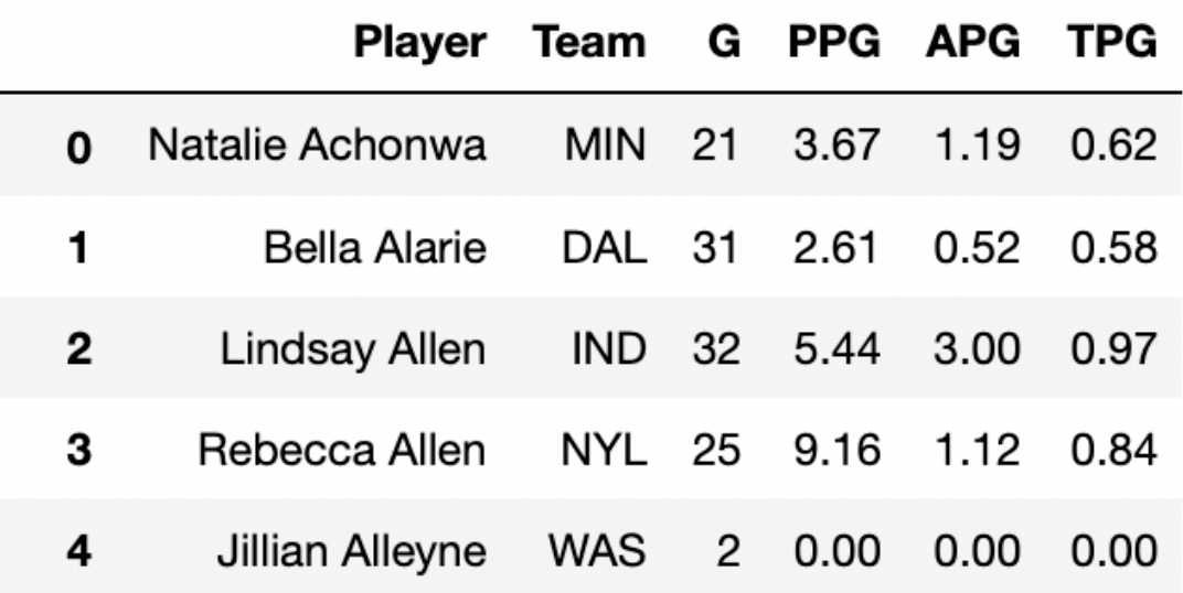
In the past three problems, we presumed that we had access to the
entire season DataFrame. Now, suppose we only have access
to the DataFrame small_season, which is a random sample of
size 36 from season. We’re interested in
learning about the true mean points per game of all players in
season given just the information in
small_season.
To start, we want to bootstrap small_season 10,000 times
and compute the mean of the resample each time. We want to store these
10,000 bootstrapped means in the array boot_means.
Here is a broken implementation of this procedure.
boot_means = np.array([])
for i in np.arange(10000):
    resample = small_season.sample(season.shape[0], replace=False)  # Line 1
    resample_mean = small_season.get('PPG').mean()                  # Line 2
    np.append(boot_means, new_mean)                                 # Line 3
For each of the 3 lines of code above (marked by comments), specify what is incorrect about the line by selecting one or more of the corresponding options below. Or, select “Line _ is correct as-is” if you believe there’s nothing that needs to be changed about the line in order for the above code to run properly.
What is incorrect about Line 1? Select all that apply.
Currently the procedure samples from small_season, when
it should be sampling from season
The sample size is season.shape[0], when it should be
small_season.shape[0]
Sampling is currently being done without replacement, when it should be done with replacement
Line 1 is correct as-is
Answers:
season.shape[0], when it should be
small_season.shape[0]Here, our goal is to bootstrap from small_season. When
bootstrapping, we sample with replacement from our
original sample, with a sample size that’s equal to the original
sample’s size. Here, our original sample is small_season,
so we should be taking samples of size
small_season.shape[0] from it.
Option 1 is incorrect; season has nothing to do with
this problem, as we are bootstrapping from
small_season.
The average score on this problem was 95%.
What is incorrect about Line 2? Select all that apply.
Currently it is taking the mean of the 'PPG' column in
small_season, when it should be taking the mean of the
'PPG' column in season
Currently it is taking the mean of the 'PPG' column in
small_season, when it should be taking the mean of the
'PPG' column in resample
.mean() is not a valid Series method, and should be
replaced with a call to the function np.mean
Line 2 is correct as-is
Answer: Currently it is taking the mean of the
'PPG' column in small_season, when it should
be taking the mean of the 'PPG' column in
resample
The current implementation of Line 2 doesn’t use the
resample at all, when it should. If we were to leave Line 2
as it is, all of the values in boot_means would be
identical (and equal to the mean of the 'PPG' column in
small_season).
Option 1 is incorrect since our bootstrapping procedure is
independent of season. Option 3 is incorrect because
.mean() is a valid Series method.
The average score on this problem was 98%.
What is incorrect about Line 3? Select all that apply.
The result of calling np.append is not being reassigned
to boot_means, so boot_means will be an empty
array after running this procedure
The indentation level of the line is incorrect –
np.append should be outside of the for-loop
(and aligned with for i)
new_mean is not a defined variable name, and should be
replaced with resample_mean
Line 3 is correct as-is
Answers:
np.append is not being reassigned
to boot_means, so boot_means will be an empty
array after running this procedurenew_mean is not a defined variable name, and should be
replaced with resample_meannp.append returns a new array and does not modify the
array it is called on (boot_means, in this case), so Option
1 is a necessary fix. Furthermore, Option 3 is a necessary fix since
new_mean wasn’t defined anywhere.
Option 2 is incorrect; if np.append were outside of the
for-loop, none of the 10,000 resampled means would be saved
in boot_means.
The average score on this problem was 94%.
Suppose we’ve now fixed everything that was incorrect about our bootstrapping implementation.
Recall from earlier in the exam that, in season, the
mean number of points per game is 7, with a standard deviation of 5.
It turns out that when looking at just the players in
small_season, the mean number of points per game is 9, with
a standard deviation of 4. Remember that small_season is a
random sample of size 36 taken from season.
Which of the following histograms visualizes the empirical distribution of the sample mean, computed using the bootstrapping procedure above?
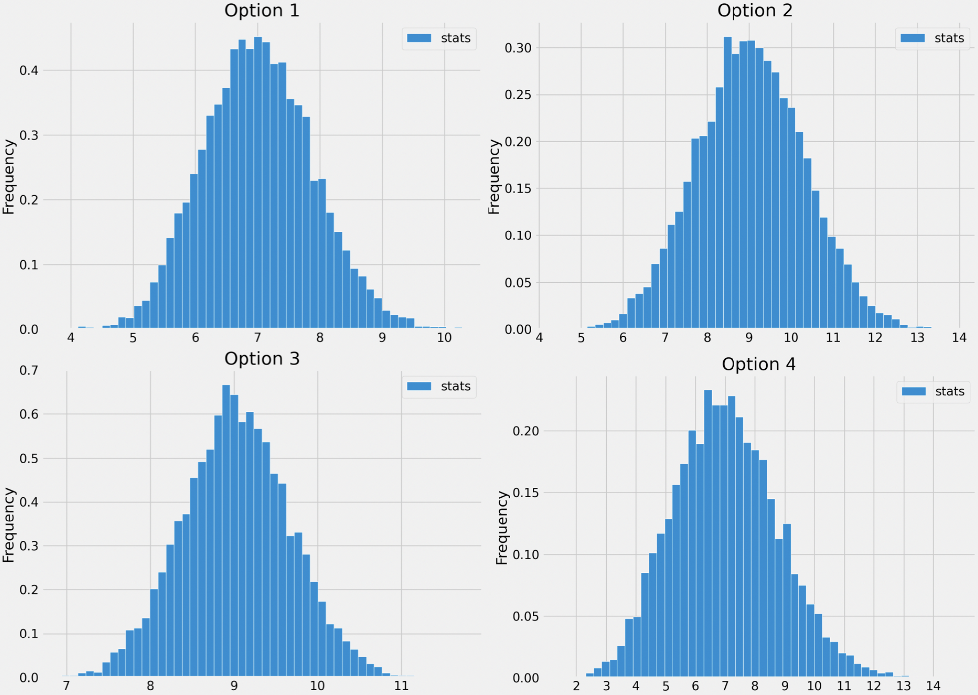
Option 1
Option 2
Option 3
Option 4
Answer: Option 3
The key to this problem is knowing to use the Central Limit Theorem. Specifically, we know that if we collect many samples from a population with replacement, then the distribution of the sample means will be roughly normal with:
Here, the “population” is small_season,
because that is the sample we’re repeatedly (re)sampling from. While
season is actually the population, it is not seen at all in
the bootstrapping process, so it doesn’t directly influence the
distribution of the bootstrapped sample means.
The mean of small_season is 9, and so is the
distribution of bootstrapped sample means. The standard deviation of
small_season is 4, so the square root law, the standard
deviation of the distribution of bootstrapped sample means is \frac{4}{\sqrt{36}} = \frac{4}{6} =
\frac{2}{3}.
The answer now boils down to choosing the histogram that looks roughly normally distributed with a mean of 9 and a standard deviation of \frac{2}{3}. Options 1 and 4 can be ruled out right away since their means seem to be smaller than 9. To decide between Options 2 and 3, we can use the inflection point rule, which states that in a normal distribution, the inflection points occur at one standard deviation above and one standard deviation below the mean. (An inflection point is when a curve changes from opening upwards to opening downwards.) See the picture below for more details.
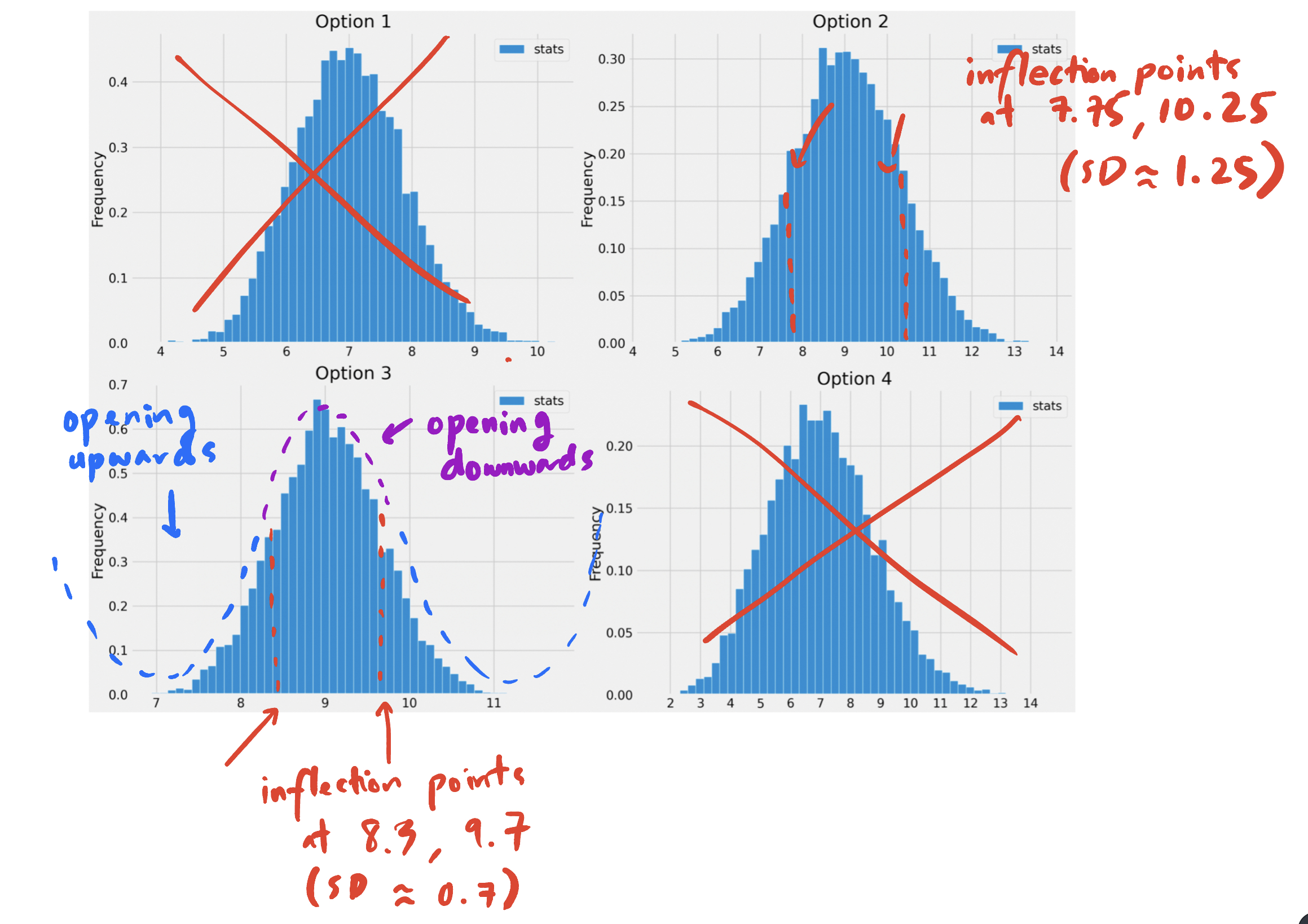
Option 3 is the only distribution that appears to be centered at 9 with a standard deviation of \frac{2}{3} (0.7 is close to \frac{2}{3}), so it must be the empirical distribution of the bootstrapped sample means.
The average score on this problem was 42%.
We construct a 95% confidence interval for the true mean points per game for all players by taking the middle 95% of the bootstrapped sample means.
left_b = np.percentile(boot_means, 2.5)
right_b = np.percentile(boot_means, 97.5)
boot_ci = [left_b, right_b]
Select the most correct statement below.
(left_b + right_b) / 2 is exactly equal to the mean
points per game in season.
(left_b + right_b) / 2 is not necessarily equal to the
mean points per game in season, but is close.
(left_b + right_b) / 2 is exactly equal to the mean
points per game in small_season.
(left_b + right_b) / 2 is not necessarily equal to the
mean points per game in small_season, but is close.
(left_b _+ right_b) / 2 is not close to either the mean
points per game in season or the mean points per game in
small_season.
Answer: (left_b + right_b) / 2 is not
necessarily equal to the mean points per game in
small_season, but is close.
Normal-based confidence intervals are of the form [\text{mean} - \text{something}, \text{mean} + \text{something}]. In such confidence intervals, it is the case that the average of the left and right endpoints is exactly the mean of the distribution used to compute the interval.
However, the confidence interval we’ve created is not normal-based, rather it is bootstrap-based! As such, we can’t say that anything is exactly true; this rules out Options 1 and 3.
Our 95% confidence interval was created by taking the middle 95% of
bootstrapped sample means. The distribution of bootstrapped sample means
is roughly normal, and the normal distribution is
symmetric (the mean and median are both equal, and represent the
“center” of the distribution). This means that the middle of our 95%
confidence interval should be roughly equal to the mean of the
distribution of bootstrapped sample means. This implies that Option 4 is
correct; the difference between Options 2 and 4 is that Option 4 uses
small_season, which is the sample we bootstrapped from,
while Option 2 uses season, which was not accessed at all
in our bootstrapping procedure.
The average score on this problem was 62%.
Instead of bootstrapping, we could also construct a 95% confidence interval for the true mean points per game by using the Central Limit Theorem.
Recall that, when looking at just the players in
small_season, the mean number of points per game is 9, with
a standard deviation of 4. Also remember that small_season
is a random sample of size 36 taken from season.
Using only the information that we have about
small_season (i.e. without using any facts about
season), compute a 95% confidence interval for the true
mean points per game.
What are the left and right endpoints of your interval? Give your answers as numbers rounded to 3 decimal places.
Answer: [7.667, 10.333]
In a normal distribution, roughly 95% of values are within 2 standard deviations of the mean. The CLT tells us that the distribution of sample means is roughly normal, and in subpart 4 of this problem we already computed the SD of the distribution of sample means to be \frac{2}{3}.
So, our normal-based 95% confidence interval is computed as follows:
\begin{aligned} &[\text{mean of sample} - 2 \cdot \text{SD of distribution of sample means}, \text{mean of sample} + 2 \cdot \text{SD of distribution of sample means}] \\ &= [9 - 2 \cdot \frac{4}{\sqrt{36}}, 9 + 2 \cdot \frac{4}{\sqrt{36}}] \\ &= [9 - \frac{4}{3}, 9 + \frac{4}{3}] \\ &\approx \boxed{[7.667, 10.333]} \end{aligned}
The average score on this problem was 87%.
Recall that the mean points per game in season is 7,
which is not in the interval you found above (if it is, check your
work!).
Select the true statement below.
The 95% confidence interval we created in the previous subpart did not contain the true mean points per game, which means that the distribution of the sample mean is not normal.
The 95% confidence interval we created in the previous subpart did
not contain the true mean points per game, which means that the
distribution of points per game in small_season is not
normal.
The 95% confidence interval we created in the previous subpart did not contain the true mean points per game. This is to be expected, because the Central Limit Theorem is only correct 95% of the time.
The 95% confidence interval we created in the previous subpart did not contain the true mean points per game, but if we collected many original samples and constructed many 95% confidence intervals, then roughly 95% of them would contain the true mean points per game.
The 95% confidence interval we created in the previous subpart did not contain the true mean points per game, but if we collected many original samples and constructed many 95% confidence intervals, then exactly 95% of them would contain the true mean points per game.
Answer: The 95% confidence interval we created in the previous subpart did not contain the true mean points per game, but if we collected many original samples and constructed many 95% confidence intervals, then roughly 95% of them would contain the true mean points per game.
In a confidence interval, the confidence level gives us a level of confidence in the process used to create the confidence interval. If we repeat the process of collecting a sample from the population and using the sample to construct a c% confidence interval for the population mean, then roughly c% of the intervals we create should contain the population mean. Option 4 is the only option that corresponds to this interpretation; the others are all incorrect in different ways.
The average score on this problem was 87%.
Suppose we sample 400 rows of olympians
at random without replacement, then generate a 95% CLT-based confidence
interval for the mean age of Olympic medalists based on this sample.
The CLT is stated for samples drawn with replacement, but in practice, we can often use it for samples drawn without replacement. What is it about this situation that makes it reasonable to still use the CLT despite the sample being drawn without replacement?
The sample is much smaller than the population.
The statistic is the sample mean.
The CLT is less computational than bootstrapping, so we don’t need to sample with replacement like we would for bootstrapping.
The population is normally distributed.
The sample standard deviation is similar to the population standard deviation.
Answer: The sample is much smaller than the population.
The Central Limit Theorem (CLT) states that regardless of the shape of the population distribution, the sampling distribution of the sample mean will be approximately normally distributed if the sample size is sufficiently large. The key factor that makes it reasonable to still use the CLT, is the sample size relative to the population size. When the sample size is much smaller than the population size, as in this case where 400 rows of Olympians are sampled from a likely much larger population of Olympians, the effect of sampling without replacement becomes negligible.
The average score on this problem was 47%.
Suppose our 95% CLT-based confidence interval for the mean age of Olympic medalists is [24.9, 26.1]. What was the mean of ages in our sample?
Answer: Mean = 25.5
We calculate the mean by first determining the width of our interval: 26.1 - 24.9 = 1.2, then we divide this width in half to get 0.6 which represents the distance from the mean to each side of the confidence interval. Using this we can find the mean in two ways: 24.9 + 0.6 = 25.5 OR 26.1 - 0.6 = 25.5.
The average score on this problem was 90%.
Suppose our 95% CLT-based confidence interval for the mean age of Olympic medalists is [24.9, 26.1]. What was the standard deviation of ages in our sample?
Answer: Standard deviation = 6
We can calculate the sample standard deviation (sample SD) by using the 95% confidence interval equation:
\text{sample mean} - 2 * \frac{\text{sample SD}}{\sqrt{\text{sample size}}}, \text{sample mean} + 2 * \frac{\text{sample SD}}{\sqrt{\text{sample size}}}.
Choose one of the end points and start plugging in all the information you have/calculated:
25.5 - 2*\frac{\text{sample SD}}{\sqrt{400}} = 24.9 → \text{sample SD} = \frac{(25.5 - 24.9)}{2}*\sqrt{400} = 6.
The average score on this problem was 55%.
We want to use the sample of data in olympians to
estimate the mean age of Olympic beach volleyball players.
Which of the following distributions must be normally distributed in order to use the Central Limit Theorem to estimate this parameter?
The age distribution of all Olympic athletes.
The age distribution of Olympic beach volleyball players.
The age distribution of Olympic beach volleyball in our sample.
None of the above.
Answer: None of the Above
The central limit theorem states that the distribution of possible sample means and sample sums is approximately normal, no matter the distribution of the population. Options A, B, and C are not probability distributions of the sum or mean of a large random sample draw with replacement.
The average score on this problem was 72%.
(10 pts) Next we want to use bootstrapping to estimate this
parameter. Which of the following code implementations correctly
generates an array called sample_means containing 10,000 bootstrapped sample means?
Way 1:
    sample_means = np.array([])
    for i in np.arange(10000):
        bv = olympians[olympians.get("Sport") == "Beach Volleyball"]
        one_mean = (bv.sample(bv.shape[0], replace=True)
                      .get("Age").mean())
        sample_means = np.append(sample_means, one_mean)
Way 2:
    sample_means = np.array([])
    for i in np.arange(10000):
        bv = olympians[olympians.get("Sport") == "Beach Volleyball"]
        one_mean = (olympians.sample(olympians.shape[0], replace=True)
                             .get("Age").mean())
        sample_means = np.append(sample_means, one_mean)
Way 3:
    sample_means = np.array([])
    for i in np.arange(10000):
        resample = olympians.sample(olympians.shape[0], replace=True)
        bv = resample[resample.get("Sport") == "Beach Volleyball"]
        one_mean = bv.get("Age").mean()
        sample_means = np.append(sample_means, one_mean)
Way 4:
    sample_means = np.array([])
    bv = olympians[olympians.get("Sport") == "Beach Volleyball"]
    for i in np.arange(10000):
        one_mean = (bv.sample(bv.shape[0], replace=True)
                      .get("Age").mean())
        sample_means = np.append(sample_means, one_mean)
Way 5:
    sample_means = np.array([])
    bv = olympians[olympians.get("Sport") == "Beach Volleyball"]
    one_mean = (bv.sample(bv.shape[0], replace=True)
                  .get("Age").mean())
    for i in np.arange(10000):
        sample_means = np.append(sample_means, one_mean)
Way 1
Way 2
Way 3
Way 4
Way 5
Answer: Way 1 and Way 4
bv, which is a subset
DataFrame of olympians but filtered to only have
"Beach Volleyball". It then samples from bv
with replacement, and counts the mean of that sample and stores it in
the variable one_sample. It does this 10,000 times (due to
the for loop), each time creating a dataframe bv, sampling
from it, calculating a mean, and then appending one_sample
to the array sample_means. This is a correct way to
bootstrap.olympians DataFrame, instead of the bv
DataFrame with only the "Beach Volleyball" players. This
will result in a sample of players of any sport, and the mean of those
ages will be calculated."Sport" column equals "Beach Volleyball" after
sampling from the DataFrame instead of before. This would lead to a mean
that is not representative of a sample of volleyball players’ ages
because we are sampling from all the rows with all different sports,
most likely resulting in a smaller sample size of volleyball players.
There would also be an inconsistent number of
"Beach Volleyball" players in each sample.bv before the for loop. The DataFrame
bv will always be the same, so it doesn’t really matter if
we make bv before or after the for loop.one_mean is calculated
only once, but is appended to the sample_means array 10,000
times. As a result, the same mean is being appended, instead of a
different mean being calculated and appended each iteration.
The average score on this problem was 88%.
For most of the answer choices in part (b), we do not have enough
information to predict how the standard deviation of
sample_means would come out. There is one answer choice,
however, where we do have enough information to compute the standard
deviation of sample_means. Which answer choice is this, and
what is the standard deviation of sample_means for this
answer choice?
Way 1
Way 2
Way 3
Way 4
Way 5
Answer: Way 5
Way 5 results in a sample_means array with the same mean appended 10,000 times. As a result the standard deviation would be 0 because the entire array would be the same value repeated.
The average score on this problem was 57%.
There are 68 rows of olympians
corresponding to beach volleyball players. Assume that in part (b), we
correctly generated an array called sample_means containing
10,000 bootstrapped sample mean ages based on this original sample of 68
ages. The standard deviation of the original sample of 68 ages is
approximately how many times larger than the standard deviation of
sample_means? Give your answer to the nearest integer.
Answer: 8
Recall SD of sample_means = \frac{\text{Population SD}}{\sqrt{\text{sample size}}}. The sample size equals 68. Based on this equation, the population SD is \sqrt{68} times larger than the SD of distribution of possible sample means. \sqrt{68} rounded to the nearest integer is 8.
The average score on this problem was 46%.
In our sample, we have data on 163 medals for the sport of table tennis. Based on our data, China seems to really dominate this sport, earning 81 of these medals.
That’s nearly half of the medals for just one country! We want to do a hypothesis test with the following hypotheses to see if this pattern is true in general, or just happens to be true in our sample.
Null: China wins half of Olympic table tennis medals.
Alternative: China does not win half of Olympic table tennis medals.
Why can these hypotheses be tested by constructing a confidence interval?
Since proportions are means, so we can use the CLT.
Since the test aims to determine whether a parameter is equal to a fixed value.
Since we need to get a sense of how other samples would come out by bootstrapping.
Since the test aims to determine if our sample came from a known population distribution.
Answer: Since the test aims to determine whether a parameter is equal to a fixed value
The goal of a confidence interval is to provide a range of values that, given the data, are considered plausible for the parameter in question. If the null hypothesis’ fixed value does not fall within this interval, it suggests that the observed data is not very compatible with the null hypothesis. Thus in our case, if a 95% confidence interval for the proportion of medals won by China does not include ~0.5, then there’s statistical evidence at the 5% significance level to suggest that China does not win exactly half of the medals. So again in our case, confidence intervals work to test this hypothesis because we are attempting to find out whether or half of the medals (0.5) lies within our interval at the 95% confidence level.
The average score on this problem was 44%.
Suppose we construct a 95% bootstrapped CI for the proportion of Olympic table tennis medals won by China. Select all true statements.
The true proportion of Olympic table tennis medals won by China has a 95% chance of falling within the bounds of our interval.
If we resampled our original sample and calculated the proportion of Olympic table tennis medals won by China in our resample, there is approximately a 95% chance our interval would contain this number.
95% of Olympic table tennis medals are won by China.
None of the above.
Answer: If we resampled our original sample and calculated the proportion of Olympic table tennis medals won by China in our resample, there is approximately a 95% chance our interval would contain this number.
The second option is the only correct answer because it accurately describes the process and interpretation of a bootstrap confidence interval. A 95% bootstrapped confidence interval means that if we repeatedly sampled from our original sample and constructed the interval each time, approximately 95% of those intervals would contain the true parameter. This statement does not imply that the true proportion has a 95% chance of falling within any single interval we construct; instead, it reflects the long-run proportion of such intervals that would contain the true proportion if we could repeat the process indefinitely. Thus, the confidence interval gives us a method to estimate the parameter with a specified level of confidence based on the resampling procedure.
The average score on this problem was 73%.
True or False: In this scenario, it would also be appropriate to create a 95% CLT-based confidence interval.
True
False
Answer: True
The statement is true because the Central Limit Theorem (CLT) applies to the sampling distribution of the proportion, given that the sample size is large enough, which in our case, with 163 medals, it is. The CLT asserts that the distribution of the sample mean (or proportion, in our case) will approximate a normal distribution as the sample size grows, allowing the use of standard methods to create confidence intervals. Therefore, a CLT-based confidence interval is appropriate for estimating the true proportion of Olympic table tennis medals won by China.
The average score on this problem was 71%.
True or False: If our 95% bootstrapped CI came out to be [0.479, 0.518], we would reject the null hypothesis at the 0.05 significance level.
True
False
Answer: False
This is false, we would fail to reject the null hypothesis because the interval [0.479, 0.518] includes the value of 0.5, which corresponds to the null hypothesis that China wins half of the Olympic table tennis medals. If the confidence interval contains the hypothesized value, there is not enough statistical evidence to reject the null hypothesis at the specified significance level. In this case, the data does not provide sufficient evidence to conclude that the proportion of medals won by China is different from 0.5 at the 0.05 significance level.
The average score on this problem was 92%.
True or False: If we instead chose to test these hypotheses at the 0.01 significance level, the confidence interval we’d create would be wider.
True
False
Answer: True
Lowering the significance level means that you require more evidence to reject the null hypothesis, thus seeking a higher confidence in your interval estimate. A higher confidence level corresponds to a wider interval because it must encompass a larger range of values to ensure that it contains the true population parameter with the increased probability. Thus as we lower the significance level, the interval we create will be wider, making this statement true.
The average score on this problem was 79%.
True or False: If we instead chose to test these hypotheses at the 0.01 significance level, we would be more likely to conclude a statistically significant result.
True
False
Answer: False
This statement is false. A small significance level lowers the chance of getting a statistically significant result; our value for 0.01 significance has to be outside a 99% confidence interval to be statistically significant. In addition, the true parameter was already contained within the tighter 95% confidence interval, so we failed to reject the null hypothesis at the 0.05 significance level. This guarantees failing to reject the null hypotehsis at the 0.01 significance level since we know that whatever is contained in a 95% confidence interval has to also be contained in a 99% confidence interval. Thus, this answer is false.
The average score on this problem was 62%.
The Oscars, or Academy Awards, are the highest awards in the film
industry, awarded each year to the best movies of that year. The
oscars DataFrame contains a row for each movie that has
ever been nominated for an Oscar. The "name" column
contains the name of the movie and the "rating" column
contains a rating of the movie on a 0 to 100 scale. This number
incorporates many factors, but we won’t worry about how it is
computed.

Fill in the blanks below to collect a simple random
sample of 400 movies from the oscars DataFrame,
then calculate 10,000 bootstrapped sample mean ratings.
my_sample = __(x)__
n_resamples = 10000
boot_means = np.array([])
for i in np.arange(n_resamples):
    resample = __(y)__
    mean = __(z)__
boot_means = np.append(boot_means, mean)Answer (x): oscars.sample(400)
The average score on this problem was 85%.
Answer (y):
my_sample.sample(400, replace=True)
The average score on this problem was 87%.
Answer (z):
resample.get("rating").mean()
The average score on this problem was 96%.
In each blank, circle the word that correctly fills in the
sentence.
A histogram of boot_means shows a(n)
probability / empirical distribution
of a statistic / parameter.
Answer: empirical, statistic
The average score on this problem was 77%.
Suppose we use the array boot_means to calculate a 90%
confidence interval for the mean rating of Oscar-nominated movies.
Select all correct conclusions we can draw about this
interval.
There is a 90% chance that the true mean rating of all Oscar-nominated movies falls within this interval.
The sample mean rating is within 90% of the true mean rating of all Oscar-nominated movies.
If we looked at the ratings of many Oscar-nominated movies, about 90% of them would fall within this range.
None of the above.
Answer: None of the above.
The average score on this problem was 74%.
Suppose both of the following expressions evaluate to
True.
my_sample.get("rating").mean() == 61.25
np.std(my_sample.get("rating")) == 15
What are the left and right endpoints of a 95% CLT-based confidence interval for the mean rating of Oscar-nominated movies?
Answer: left endpoint: 59.75, right endpoint: 62.75
The average score on this problem was 54%.
Among Hogwarts students, Chocolate Frogs are a popular enchanted treat. Chocolate Frogs are individually packaged, and every Chocolate Frog comes with a collectible card of a famous wizard (ex.”Albus Dumbledore"). There are 80 unique cards, and each package contains one card selected uniformly at random from these 80.
Neville would love to get a complete collection with all 80 cards, and he wants to know how many Chocolate Frogs he should expect to buy to make this happen.

Suppose we have access to a function called
frog_experiment that takes no inputs and simulates the act
of buying Chocolate Frogs until a complete collection of cards is
obtained. The function returns the number of Chocolate Frogs that were
purchased. Fill in the blanks below to run 10,000 simulations and set
avg_frog_count to the average number of Chocolate Frogs
purchased across these experiments.
    frog_counts = np.array([])

    for i in np.arange(10000):
        frog_counts = np.append(__(a)__)

avg_frog_count = __(b)__What goes in blank (a)?
Answer:
frog_counts, frog_experiment()
Each call to frog_experiment() simulates purchasing
Chocolate Frogs until a complete set of 80 unique cards is obtained,
returning the total number of frogs purchased in that simulation. The
result of each simulation is then appended to the
frog_counts array.
The average score on this problem was 65%.
What goes in blank (b)?
Answer: frog_counts.mean()
After running the loop for 10000 times, the frog_counts
array holds all the simulated totals. Taking the mean of that array
(frog_counts.mean()) gives the average number of frogs
needed to complete the set of 80 unique cards.
The average score on this problem was 89%.
Realistically, Neville can only afford to buy 300 Chocolate Frog
cards. Using the simulated data in frog_counts, write a
Python expression that evaluates to an approximation of the probability
that Neville will be able to complete his collection.
Answer:
np.count_nonzero(frog_counts <= 300) / len(frog_counts)
or equivlent, such as
np.count_nonzero(frog_counts <= 300) / 10000 or
(frog_counts <= 300).mean()
In the simulated data, each entry of frog_counts is the
number of Chocolate Frogs purchased in one simulation before collecting
all 80 unique cards. We want to estimate the probability that Neville
completes his collection with at most 300 cards.
frog_counts <= 300 creates a boolean array of the
same length as frog_counts, where each element is True if
the number of frogs used in that simulation was 300 or fewer, and False
otherwise.
np.count_nonzero(frog_counts <= 300) counts how many
simulations (out of all the simulations) met the condition since
True evaluates to 1 and False evaluates to
0.
Dividing by the total number of simulations,
len(frog_counts), converts that count to probability.
The average score on this problem was 59%.
True or False: The Central Limit Theorem states that
the data in frog_counts is roughly normally
distributed.
True
False
Answer: False
The Central Limit Theorem (CLT) says that the probability distribution of the sum or mean of a large random sample drawn with replacement will be roughly normal, regardless of the distribution of the population from which the sample is drawn.
The Central Limit Theorem (CLT) does not claim that individual
observations are normally distributed. In this problem, each entry of
frog_counts is a single observation: the number of frogs
purchased in one simulation to complete the collection. There is no
requirement that these individual data points themselves follow a normal
distribution.
However, if we repeatedly take many samples of such observations and compute the sample mean, then that mean would tend toward a normal distribution as the sample size grows, follows the CLT.
The average score on this problem was 38%.
The DataFrame geisel contains a row for each day of this
academic year. The "Students" column contains the number of
students who visited Geisel Library on that day, as an
int.
Fill in the blanks below such that
geisel_sample is a simple random
sample of 50 rows of geisel, and
the code prints the endpoints of a 95% bootstrapped confidence
interval for the mean number of students at Geisel
Library, based on the data in geisel_sample.
    geisel_sample = __(a)___
    y = np.array([]):
    for i in np.arange(10000):
        x = __(b)__
        y = np.append(y, x)
print(np.percentile(y, 2.5), np.percentile(y, 97.5))Answer (a): geisel.sample(50) or
geisel.sample(50, replace = False)
Answer (b):
geisel_sample.sample(50, replace = True).get("Students").mean()
or equivalent
The average score on this problem was 75%.
Which of the following is the best description of x and
y in the code above?
x represents the original sample, and y
represents many resamples.
x represents the average student count for a single day,
and y represents the student count on all days.
x represents the sample statistic from a single
resample, and y represents the distribution of those
statistics across multiple resamples.
x represents the sample statistic for the original
sample, and y represents a distribution of statistics
across multiple resamples.
x represents the population parameter, and
y represents a bootstrapped distribution of sample
statistics.
Answer: Option 3: x represents the
sample statistic from a single resample, and y represents
the distribution of those statistics across multiple resamples.
The average score on this problem was 72%.
Select all true statements below.
If geisel_sample had instead had 60 rows, the resulting 95\% confidence interval would have been
wider.
If we made 100 95\% confidence intervals based on
geisel_sample, about 95 of
them would contain the population mean.
On about 95\% of days, the number of students at Geisel Library falls between the endpoints of our confidence interval.
It would have also been appropriate to generate a confidence interval for this parameter using the Central Limit Theorem.
The standard deviation of geisel_sample should be
approximately the same as the standard deviation of
geisel
The data in geisel_sample is roughly normally
distributed.
Answer:
Option 4: It would have also been appropriate to generate a confidence interval for this parameter using the Central Limit Theorem.
Option 5: The standard deviation of geisel_sample should
be approximately the same as the standard deviation of
geisel
The average score on this problem was 69%.