← return to practice.dsc10.com
Below are practice problems tagged for Lecture 20 (rendered directly from the original exam/quiz sources).
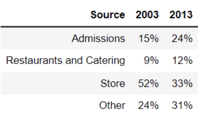
The table below shows the average amount of revenue from different sources for art museums in 2003 and 2013.
What is the total variation distance between the distribution of revenue sources in 2003 and the distribution of revenue sources in 2013? Give your answer as a proportion (i.e. a decimal between 0 and 1), not a percentage. Round your answer to three decimal places.
Answer: 0.19
Recall, the total variation distance (TVD) is the sum of the absolute differences in proportions, divided by 2. The absolute differences in proportions for each source are as follows:
Then, we have
\text{TVD} = \frac{1}{2} (0.09 + 0.03 + 0.19 + 0.07) = 0.19
The average score on this problem was 95%.
Which type of visualization would be best suited for comparing the two distributions in the table?
Scatter plot
Line plot
Overlaid histogram
Overlaid bar chart
Answer: Overlaid bar chart
A scatter plot visualizes the relationship between two numerical variables. In this problem, we only have to visualize the distribution of a categorical variable.
A line plot shows trends in numerical variables over time. In this problem, we only have categorical variables. Moreover, when it says over time, it is suitable for plotting change in multiple years (e.g. 2001, 2002, 2003, … , 2013), or even with data of days. In this question, we only want to compare the distribution of 2003 and 2013, this makes the line plot not useful. In addition, if you try to draw a line plot for this question, you will find the line plot fails to visualize distribution (e.g. the idea of 15%, 9%, 52%, and 24% add up to 100%).
An overlaid graph is useful in this question since this visualizes comparison between the two distributions.
However, an overlaid histogram is not useful in this problem. The key reason is the differences between a histogram and a bar chart.
Bar Chart: Space between the bars; 1 categorical axis, 1 numerical
axis; order does not matter
Histogram: No space between the bars; intervals on axis; 2 numerical
axes; order matters
In the question, we are plotting 2003 and 2013 distributions of four categories (Admissions, Restaurants and Catering, Store, and Other). Thus, an overlaid bar chart is more appropriate.
The average score on this problem was 74%.
Note: This problem is out of scope; it covers material no longer included in the course.
Notably, there was an economic recession in 2008-2009. Which of the following can we conclude was an effect of the recession?
The increase in revenue from admissions, as more people were visiting museums.
The decline in revenue from museum stores, as people had less money to spend.
The decline in total revenue, as fewer people were visiting museums.
None of the above
Answer: None of the above
Since we are only given the distribution of the revenue, and have no information about the amount of revenue in 2003 and 2013, we cannot conclude how the revenue has changed from 2003 to 2013 after the recession.
For instance, if the total revenue in 2003 was 100 billion USD and the total revenue in 2013 was 50 billion USD, revenue from admissions in 2003 was 100 * 15% = 15 billion USD, and revenue from admissions in 2003 was 50 * 24% = 12 billion USD. In this case, we will have 15 > 12, the revenue from admissions has declined rather than increased (As stated by ‘The increase in revenue from admissions, as more people were visiting museums.’). Similarly, since we don’t know the total revenue in 2003 and 2013, we cannot conclude ‘The decline in revenue from museum stores, as people had less money to spend.’ or ‘The decline in total revenue, as fewer people were visiting museums.’
The average score on this problem was 72%.
For each application in apps, we want to assign an age
category based on the value in the "age" column, according
to the table below.
"age" |
age category |
|---|---|
| under 25 | "young adult" |
| at least 25, but less than 50 | "middle aged" |
| at least 50, but less than 75 | "older adult" |
| 75 or over | "elderly" |
cat_names = ["young adult", "middle aged", "older adult", "elderly"]

def age_to_bin(one_age):
    '''Returns the age category corresponding to one_age.'''
    one_age = __(a)__
    bin_pos = __(b)__
    return cat_names[bin_pos]

binned_ages = __(c)__
apps_cat = apps.assign(age_category = binned_ages)Which of the following is a correct way to fill in blanks (a) and (b)?
| Blank (a) | Blank (b) | |
|---|---|---|
| Option 1 | 75 - one_age |
round(one_age / 25) |
| Option 2 | min(75, one_age) |
one_age / 25 |
| Option 3 | 75 - one_age |
int(one_age / 25) |
| Option 4 | min(75, one_age) |
int(one_age / 25) |
| Option 5 | min(74, one_age) |
round(one_age / 25) |
Option 1
Option 2
Option 3
Option 4
Option 5
Answer: Option 4
The line one_age = min(75, one_age) either leaves
one_age alone or sets it equal to 75 if the age was higher
than 75, which means anyone over age 75 is considered to be 75 years old
for the purposes of classifying them into age categories. From the
return statement, we know we need our value for bin_pos to
be either 0, 1 ,2 or 3 since cat_names has a length of 4.
When we divide one_age by 25, we get a decimal number that
represents how many times 25 fits into one_age. We want to
round this number down to get the number of whole copies of 25
that fit into one_age. If that value is 0, it means the
person is a "young adult", if that value is 1, it means
they are "middle aged", and so on. The rounding down
behavior that we want is accomplished by
int(one_age/25).
The average score on this problem was 76%.
Which of the following is a correct way to fill in blank (c)?
age to bin(apps.get("age"))
apps.get("age").apply(age to bin)
apps.get("age").age to bin()
apps.get("age").apply(age to bin(one age))
Answer:
apps.get("age").apply(age to bin)
We want our result to be a Series because the next line in the code
assigns it to a DataFrame. We also need to use the .apply()
method to apply our function to the entirety of the "age"
column. The .apply() method only takes in the name of a
function and not its variables, as it treats the entries of the column
as the variables directly.
The average score on this problem was 96%.
Which of the following is a correct alternate implementation of the age to bin function? Select all that apply.
Option 1:
def age_to_bin(one_age):
    bin_pos = 3
    if one_age < 25:
        bin_pos = 0
    if one_age < 50:
        bin_pos = 1
    if one_age < 75:
        bin_pos = 2
    return cat_names[bin_pos]
Option 2:
def age_to_bin(one_age):
    bin_pos = 3
    if one_age < 75:
        bin_pos = 2
    if one_age < 50:
        bin_pos = 1
    if one_age < 25:
        bin_pos = 0
    return cat_names[bin_pos]
Option 3:
def age_to_bin(one_age):
    bin_pos = 0
    for cutoff in np.arange(25, 100, 25):
        if one_age >= cutoff:
            bin_pos = bin_pos + 1
    return cat_names[bin_pos]
Option 4:
def age_to_bin(one_age):
    bin_pos = -1
    for cutoff in np.arange(0, 100, 25):
        if one_age >= cutoff:
            bin_pos = bin_pos + 1
        return cat_names[bin_pos]
Option 1
Option 2
Option 3
Option 4
None of the above.
Answer: Option 2 and Option 3
Option 1 doesn’t work for inputs less than 25. For example, on an
input of 10, every condition is satsified, so bin_pos will
be set to 0, then 1, then 2, meaning the function will return
"older adult" instead of "young adult".
Option 2 reverses the order of the conditions, which ensures that
even when a number satisfies many conditions, the last one it satisfies
determines the correct bin_pos. For example, 27 would
satisfy the first 2 conditions but not the last one, and the function
would return "middle aged" as expected.
In option 3, np.arange(25, 100, 25) produces
np.array([25,50,75]). The if condition checks
the whether the age is at least 25, then 50, then 75. For every time
that it is, it adds to bin_pos, otherwise it keeps
bin_pos. At the end, bin_pos represents the
number of these values that the age is greater than or equal to, which
correctly determines the age category.
Option 4 is equivalent to option 3 except for two things. First,
bin_pos starts at -1, but since 0 is included in the set of
cutoff values, the first time through the loop will set
bin_pos to 0, as in Option 3. This change doesn’t affect
the behavior of the funtion. The other change, however, is that the
return statement is inside the for-loop, which
does change the behavior of the function dramatically. Now the
for-loop will only run once, checking whether the age is at
least 0 and then returning immediately. Since ages are always at least
0, this function will return "young adult" on every input,
which is clearly incorrect.
The average score on this problem was 62%.
We want to determine the number of "middle aged"
applicants whose applications were denied. Fill in the blank below so
that count evaluates to that number.
df = apps_cat.________.reset_index()
count = df[(df.get("age_category") == "middle aged") &
           (df.get("status") == "denied")].get("income").iloc[0]
What goes in the blank?
Answer:
groupby(["age_category", "status"]).count()
We can tell by the line in which count is defined that
df needs to have columns called
"age category", "status", and
"income" with one row such that the values in these columns
are "middle aged", "denied", and the number of
such applicants, respectively. Since there is one row corresponding to a
possible combination of values for "age category" and
"status", this suggests we need to group by the pair of
columns, since .groupby produces a DataFrame with one row
for each possible combination of values in the columns we are grouping
by. Since we want to know how many individuals have this combination of
values for "age category" and "status", we
should use .count() as the aggregation method. Another clue
to to use .groupby is the presence of
.reset_index() which is needed to query based on columns
called "age category" and "status".
The average score on this problem was 78%.
The total variation distance between the distributions of
"age category" for approved applications and denied
applications is 0.4.
One of the visualizations below shows the distributions of
"age category" for approved applications and denied
applications. Which visualization is it?
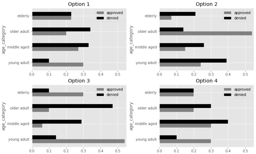
Answer: Option 2
TVD represents the total overrepresentation of one distrubtion, summed across all categories. To find the TVD visually, we can estimate how much each bar for approved applications extends beyond the corresponding bar for denied applications in each bar chart.
In Option 1, the approved bar extends beyond the denied bar only in
the "young adult" category, and by 0.2, so the TVD for
Option 1 is 0.2. In Option 2, the approved bar extends beyond the denied
bar only in the "older adult" category, and by 0.4, so the
TVD for Option 2 is 0.4. In Option 3, the approved bar extends beyond
the denied bar in "elderly" by 0.2 and in
"young adult" by 0.4, for a TVD of 0.6. In Option 4, the
approved bar extends beyond the denied bar in
"young adult only" by 0.2, for a TVD of 0.2.
Note that even without knowing the exact lengths of the bars in Option 2, we can still conclude that Option 2 is correct by process of elimination, since it’s the only one whose TVD appears close to 0.4
The average score on this problem was 60%.
Aaron wants to explore the discrepancy in fraud rates between
"discover" transactions and "mastercard"
transactions. To do so, he creates the DataFrame ds_mc,
which only contains the rows in txn corresponding to
"mastercard" or "discover" transactions.
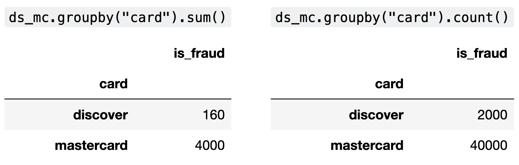
After he creates ds_mc, Aaron groups ds_mc
on the "card" column using two different aggregation
methods. The relevant columns in the resulting DataFrames are shown
below.
Aaron decides to perform a test of the following pair of hypotheses:
Null Hypothesis: The proportion of fraudulent
"mastercard" transactions is the same as
the proportion of fraudulent "discover"
transactions.
Alternative Hypothesis: The proportion of
fraudulent "mastercard" transactions is less
than the proportion of fraudulent "discover"
transactions.
As his test statistic, Aaron chooses the difference in
proportion of transactions that are fraudulent, in the order
"mastercard" minus "discover".
What type of statistical test is Aaron performing?
Standard hypothesis test
Permutation test
Answer: Permutation test
Permutation tests are used to ascertain whether two samples were
drawn from the same population. Hypothesis testing is used when we have
a single sample and a known population, and want to determine whether
the sample appears to have been drawn from that population. Here, we
have two samples (“mastercard” and “discover”)
and no known population distribution, so a permutation test is the
appropriate test.
The average score on this problem was 49%.
What is the value of the observed statistic? Give your answer either as an exact decimal or simplified fraction.
Answer: 0.02
We simply take the difference in fraudulent proportion of
"mastercard" transactions and fraudulent proportion of
discover transactions. There are 4,000 fraudulent
"mastercard" transactions and 40,000 total
"mastercard" transactions, making this proportion for
"mastercard". Similarly, the proportion of fraudulent
"discover" transactions is \frac{160}{2000}. Simplifying these
fractions, the difference between them is \frac{1}{10} - \frac{8}{100} = 0.1 - 0.08 =
0.02.
The average score on this problem was 86%.
The empirical distribution of Aaron’s chosen test statistic is shown below.
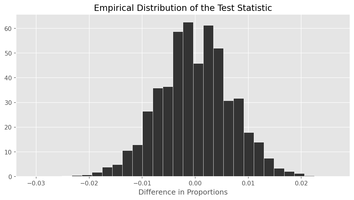
Which of the following is closest to the p-value of Aaron’s test?
0.001
0.37
0.63
0.94
0.999
Answer: 0.999
Informally, the p-value is the area of the histogram at or past the
observed statistic, further in the direction of the alternative
hypothesis. In this case, the alternative hypothesis is that the
"mastercard" proportion is less than the discover
proportion, and our test statistic is computed in the order
"mastercard" minus "discover", so low
(negative) values correspond to the alternative. This means when
calculating the p-value, we look at the area to the left of 0.02 (the
observed value). We see that essentially all of the test statistics fall
to the left of this value, so the p-value should be closest to
0.999.
The average score on this problem was 54%.
What is the conclusion of Aaron’s test?
The proportion of fraudulent "mastercard" transactions
is less than the proportion of fraudulent
"discover" transactions.
The proportion of fraudulent "mastercard" transactions
is greater than the proportion of fraudulent
"discover" transactions.
The test results are inconclusive.
None of the above.
Answer: None of the above
"mastercard" transactions is less
than the proportion of fraudulent "discover" transactions,
so we cannot conclude A.
The average score on this problem was 44%.
Aaron now decides to test a slightly different pair of hypotheses.
Null Hypothesis: The proportion of fraudulent
"mastercard" transactions is the same as
the proportion of fraudulent "discover"
transactions.
Alternative Hypothesis: The proportion of
fraudulent "mastercard" transactions is greater
than the proportion of fraudulent "discover"
transactions.
He uses the same test statistic as before.
Which of the following is closest to the p-value of Aaron’s new test?
0.001
0.06
0.37
0.63
0.94
0.999
Answer: 0.001
Now, we have switched the alternative hypothesis to “
"mastercard" fraud rate is greater than
"discover" fraud rate”, whereas before our alternative
hypothesis was that the "mastercard" fraud rate was less
than "discover"’s fraud rate. We have not changed the way
we calculate the test statistic ("mastercard" minus
"discover"), so now large values of the test statistic
correspond to the alternative hypothesis. So, the area of interest is
the area to the right of 0.02, which is very small, close to 0.001. Note
that this is one minus the p-value we computed before.
The average score on this problem was 65%.
Jason is interested in exploring the relationship between the browser
and payment method used for a transaction. To do so, he uses
txn to create create three tables, each of which contain
the distribution of browsers used for credit card transactions and the
distribution of browsers used for debit card transactions, but with
different combinations of browsers combined in a single category in each
table.
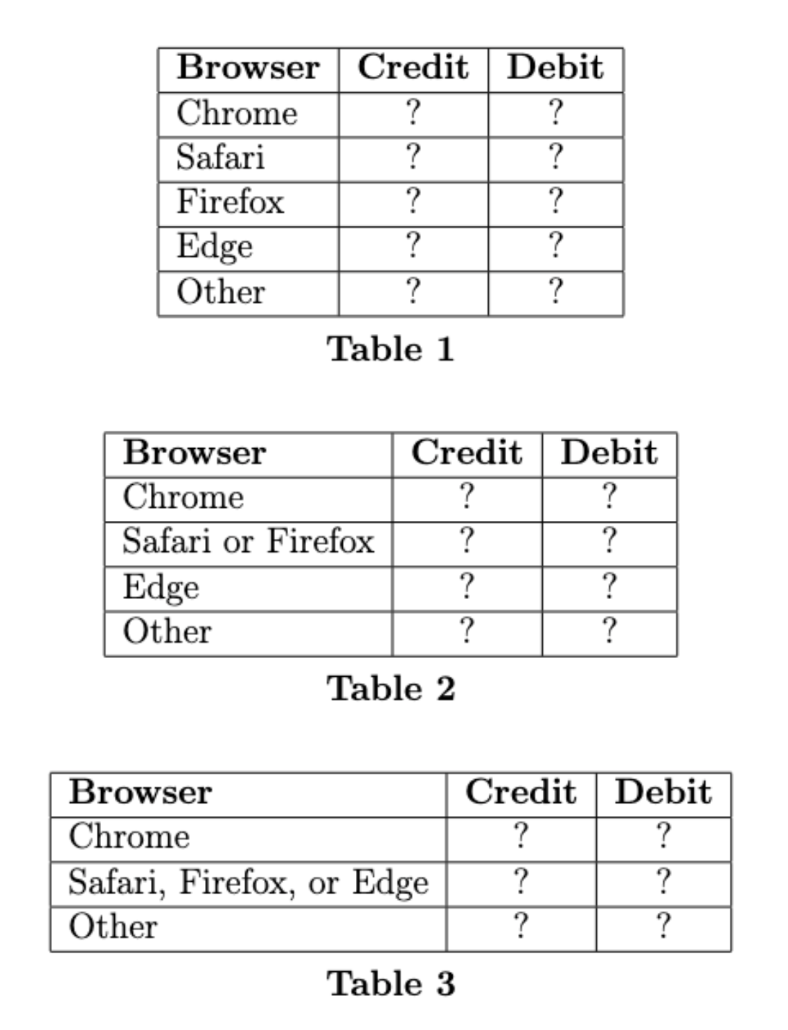
Jason calculates the total variation distance (TVD) between the two distributions in each of his three tables, but he does not record which TVD goes with which table. He computed TVDs of 0.14, 0.36, and 0.38.
In which table do the two distributions have a TVD of 0.14?
Table 1
Table 2
Table 3
Answer: Table 3
Without values in any of the tables, there’s no way to do this problem computationally. We are told that the three TVDs come out to 0.14, 0.36, and 0.38. The exact numbers are not important but their relative order is. The key to this problem is noticing that when we combine two categories into one, the TVD can only decrease, it cannot increase. One way to see this is to think about combining categories repeatedly until there’s just one category. Then both distributions must have a value of 1 in that category so they are identical distributions with the smallest possible TVD of 0. As we collapse categories, we can only decrease the TVD. This tells us that Table 1 has the largest TVD, then Table 2 has the middle TVD, and Table 3 has the smallest, since each time we are combining categories and shrinking the TVD.
The average score on this problem was 77%.
In which table do the two distributions have a TVD of 0.36?
Table 1
Table 2
Table 3
Answer: Table 2
See the solution to 7.1.
The average score on this problem was 97%.
In which table do the two distributions have a TVD of 0.38?
Table 1
Table 2
Table 3
Answer: Table 1
See the solution to 7.1.
The average score on this problem was 77%.
You survey 100 DSC majors and 140 CSE majors to ask them which video streaming service they use most. The resulting distributions are given in the table below. Note that each column sums to 1.
| Service | DSC Majors | CSE Majors |
|---|---|---|
| Netflix | 0.4 | 0.35 |
| Hulu | 0.25 | 0.2 |
| Disney+ | 0.1 | 0.1 |
| Amazon Prime Video | 0.15 | 0.3 |
| Other | 0.1 | 0.05 |
For example, 20% of CSE Majors said that Hulu is their most used video streaming service. Note that if a student doesn’t use video streaming services, their response is counted as Other.
What is the total variation distance (TVD) between the distribution for DSC majors and the distribution for CSE majors? Give your answer as an exact decimal.
Answer: 0.15
The average score on this problem was 89%.
Suppose we only break down video streaming services into four categories: Netflix, Hulu, Disney+, and Other (which now includes Amazon Prime Video). Now we recalculate the TVD between the two distributions. How does the TVD now compare to your answer to part (a)?
less than (a)
equal to (a)
greater than (a)
Answer: less than (a)
The average score on this problem was 93%.
Arya was curious how many UCSD students used Hulu over Thanksgiving break. He surveys 250 students and finds that 130 of them did use Hulu over break and 120 did not.
Using this data, Arya decides to test following hypotheses:
Null Hypothesis: Over Thanksgiving break, an equal number of UCSD students did use Hulu and did not use Hulu.
Alternative Hypothesis: Over Thanksgiving break, more UCSD students did use Hulu than did not use Hulu.
Which of the following could be used as a test statistic for the hypothesis test?
The proportion of students who did use Hulu minus the proportion of students who did not use Hulu.
The absolute value of the proportion of students who did use Hulu minus the proportion of students who did not use Hulu.
The proportion of students who did use Hulu plus the proportion of students who did not use Hulu.
The absolute value of the proportion of students who did use Hulu plus the proportion of students who did not use Hulu.
Answer: The proportion of students who did use Hulu minus the proportion of students who did not use Hulu.
The average score on this problem was 81%.
For the test statistic that you chose in part (a), what is the observed value of the statistic? Give your answer either as an exact decimal or a simplified fraction.
Answer: 0.04
The average score on this problem was 90%.
If the p-value of the hypothesis test is 0.053, what can we conclude, at the standard 0.05 significance level?
We reject the null hypothesis.
We fail to reject the null hypothesis.
We accept the null hypothesis.
Answer: We fail to reject the null hypothesis.
The average score on this problem was 87%.
Hargen is an employee at Bill’s Book Bonanza who tends to work weekend shifts. He thinks that Fridays, Saturdays, and Sundays are busier than other days, and he proposes the following probability distribution of sales by day:
| Sunday | Monday | Tuesday | Wednesday | Thursday | Friday | Saturday |
|---|---|---|---|---|---|---|
| 0.2 | 0.1 | 0.1 | 0.1 | 0.1 | 0.2 | 0.2 |
Let’s use the data in sales to determine whether
Hargen’s proposed model could be correct by doing a hypothesis test. The
hypotheses are:
Null Hypothesis: Sales at the bookstore are randomly drawn from Hargen’s proposed distribution of days.
Alternative Hypothesis: Sales at the bookstore are not randomly drawn from Hargen’s proposed distribution of days.
Which of the following test statistics could be used to test the given hypothesis? Select all that apply.
The absolute difference between the proportion of books sold on Saturday and the proposed proportion of books sold on Saturday (0.2).
The sum of the differences in proportions between the distribution of books sold by day and Hargen’s proposed distribution.
The sum of the squared differences in proportions between the distribution of books sold by day and Hargen’s proposed distribution.
One half of the sum of the absolute differences in proportions between the distribution of books sold by day and Hargen’s proposed distribution.
Answer:
Let’s look at each of the options:
The average score on this problem was 74%.
We will use as our test statistic the mean of the absolute differences in proportions between the distribution of books sold by day and Hargen’s proposed distribution.
Suppose the observed distribution of books sold by day was as follows. Calculate the observed statistic in this case.
| Sunday | Monday | Tuesday | Wednesday | Thursday | Friday | Saturday |
|---|---|---|---|---|---|---|
| 0.34 | 0.13 | 0.06 | 0.07 | 0.08 | 0.08 | 0.24 |
Answer: 0.06
\begin{align*} \text{mean abs diff} &= \frac{|0.34 - 0.2| + |0.13 - 0.1| + |0.06 - 0.1| + |0.07 - 0.1| + |0.08 - 0.1| + |0.08 - 0.2| + |0.24 - 0.2|}{7}\\ &= \frac{0.14 + 0.03 + 0.04 + 0.03 + 0.02 + 0.12 + 0.04}{7}\\ &= \frac{0.42}{7} \\ &= 0.06 \end{align*}
The average score on this problem was 69%.
Let’s determine the actual value of the observed statistic based on
the data in sales. Assume that we have already defined a
function called find_day that returns the day of the week
for a given "date". For example,
find_day("Saturday, December 7, 2024") evaluates to
"Saturday". Fill in the blanks below so that the variable
obs evaluates to the observed statistic.
# in alphabetical order: Fri, Mon, Sat, Sun, Thurs, Tues, Wed
hargen = np.array([0.2, 0.1, 0.2, 0.2, 0.1, 0.1, 0.1])
prop = (sales.assign(day_of_week = __(a)__)
             .groupby(__(b)__).__(c)__.get("ISBN") / sales.shape[0])
obs = __(d)__(a). Answer:
sales.get("date").apply(find_day)
In this blank, we want to create a Series that contains days of the
week, such as "Saturday", to be assigned to a column named
day_of_week in sales. We take the
"date" column in sales and apply the function
find_day to each of the date in the column.
The average score on this problem was 77%.
(b). Answer: "day_of_week"
We want to group the sales DataFrame by the
day_of_week column that was created in blank (a) to collect
together all rows corresponding to the same day of the week.
The average score on this problem was 84%.
(c). Answer: count()
We want to count how many sales occurred on each day of the week, or,
how many rows are in sales that belong to each day, so we
use count() after grouping by day_of_week.
The average score on this problem was 71%.
(d). Answer:
(np.abs(prop - hargen)).mean()
We first take one column that contains the count of rows for each day
of the week, indexed by the days in alphabetical order after the
groupby. We then divide this column by the total number of rows to get
proportions. We want to compute the statistic that we’ve chosen, the
mean of absolute differences in proportions between the observed and
Hargen’s proposed distribution. Since the order of the days already
match (both in alphabetical order), we can simply subtract one from the
other to get the difference in proportions. We then turn the differences
into absolute differences with np.abs and get the mean
using .mean().
The average score on this problem was 59%.
To conduct the hypothesis test, we’ll need to generate thousands of simulated day-of-the-week distributions. What will we do with all these simulated distributions?
Use them to determine whether Hargen’s proposed distribution looks like a typical simulated distribution.
Use them to determine whether the observed distribution of books sold by day looks like a typical simulated distribution.
Use them to determine whether Hargen’s proposed distribution looks like a typical observed distribution of books sold by day.
Answer: Use them to determine whether the observed distribution of books sold by day looks like a typical simulated distribution.
For hypothesis testing, we simulate based on the null distribution, which is the distribution that Hargen proposed. For each of the simulated distribution of proportions , we calculate the statistic we chose. After many simulations, we have calculated thousands of these statistics, each between one simulated distribution and Hargen’s proposed distribution. Lastly, we compare the observed statistic with the statistics from the simulations to see whether the observed distribution of books sold by day looks like a typical simulated distribution.
The average score on this problem was 28%.
In each iteration of the simulation, we need to collect a sample of
size sales.shape[0] from which distribution?
Hargen’s proposed distribution.
The distribution of data in sales by day of the
week.
Our original sample’s distribution.
The distribution of possible sample means.
Answer: Hargen’s proposed distribution.
For hypothesis testing, we simulate based on the null distribution, which is the distribution that Hargen proposed.
The average score on this problem was 26%.
Suppose that obs comes out to be in the 98th percentile
of simulated test statistics. Using the standard p-value cutoff of 0.05,
what would Hargen conclude about his original model?
It is likely correct.
It is plausible.
It is likely wrong.
Answer: It is likely wrong.
Using the standard p-value cutoff of 0.05, we say that the observed distribution is not like a typical simulated distribution under Hargen’s proposed distribution if it falls below 2.5th percentile of above 97.5th percentile. In this case, 98th percentile is above 97.5th percentile, so we say that Hargen’s proposed distribution is likely wrong.
The average score on this problem was 63%.
Suppose the bookstore DataFrame has 10 unique genres, and we are given a sample
of 350 books from that DataFrame.
Determine the maximum possible total variation distance (TVD) that could
occur between our sample’s genre distribution and the uniform
distribution where each genre occurs with equal probability. Your answer
should be a single number.
Answer: 0.9
To determine the maximum possible TVD, we consider the scenario where all books belong to a single genre. This represents the maximum deviation from the uniform distribution:
TVD = \frac{1}{2} \left( |1 - 0.1| + 9 \times |0 - 0.1| \right) = \frac{1}{2} (0.9 + 0.9) = 0.9
The average score on this problem was 31%.
True or False: If the sample instead had 700 books, then the maximum possible TVD would increase.
True
False
Answer: False
The maximum possible TVD is based on proportions and not absolute counts. Even if the sample size is increased, the TVD would remain the same.
The average score on this problem was 71%.
True or False: If the bookstore DataFrame had 11 genres
instead of 10, the maximum possible TVD would
increase.
True
False
Answer: True
With 11 genres, the uniform probability per genre decreases to \frac{1}{11} instead of \frac{1}{10} with 10 genres. In the extreme scenario where one genre dominates, the TVD is now bigger.
TVD = \frac{1}{2} \left( |1 - \frac{1}{11}| + 10 \times |0 - \frac{1}{11}| \right) = \frac{1}{2} (\frac{10}{11} + \frac{10}{11}) = \frac{10}{11}
The average score on this problem was 66%.
Calculate the TVD between the two distributions in the
soxcards DataFrame.
Answer: 0.11
The average score on this problem was 83%.
Suppose we were to split the "IF" group into all of its
individual positions and their respective proportions. How might the TVD
change? Select all that could be true.
Increase
Decrease
Stay the same
Answer: Options 1 and 3
The average score on this problem was 74%.
There are 52 IKEA locations in the United States, and there are 50 states.
Which of the following describes how to calculate the total variation distance between the distribution of IKEA locations by state and the uniform distribution?
For each IKEA location, take the absolute difference between 1/50 and the number of IKEAs in the same state divided by the total number of IKEA locations. Sum these values across all locations and divide by two.
For each IKEA location, take the absolute difference between the number of IKEAs in the same state and the average number of IKEAs in each state. Sum these values across all locations and divide by two.
For each state, take the absolute difference between 1/50 and the number of IKEAs in that state divided by the total number of IKEA locations. Sum these values across all states and divide by two.
For each state, take the absolute difference between the number of IKEAs in that state and the average number of IKEAs in each state. Sum these values across all states and divide by two.
None of the above.
Answer: For each state, take the absolute difference between 1/50 and the number of IKEAs in that state divided by the total number of IKEA locations. Sum these values across all states and divide by two.
We’re looking at the distribution across states. Since there are 50 states, the uniform distribution would correspond to having a fraction of 1/50 of the IKEA locations in each state. We can picture this as a sequence with 50 entries that are all the same: (1/50, 1/50, 1/50, 1/50, \dots)
We want to compare this to the actual distribution of IKEAs across states, which we can think of as a sequence with 50 entries, representing the 50 states, but where each entry is the proportion of IKEA locations in a given state. For example, maybe the distribution starts out like this: (3/52, 1/52, 0/52, 1/52, \dots) We can interpret each entry as the number of IKEAs in a state divided by the total number of IKEA locations. Note that this has nothing to do with the average number of IKEA locations in each state, which is 52/50.
The way we take the TVD of two distributions is to subtract the distributions, take the absolute value, sum up the values, and divide by 2. Since the entries represent states, this process aligns with the given answer.
The average score on this problem was 30%.
For this question, let’s think of the data in app_data
as a random sample of all IKEA purchases and use it to test the
following hypotheses.
Null Hypothesis: IKEA sells an equal amount of beds
(category 'bed') and outdoor furniture (category
'outdoor').
Alternative Hypothesis: IKEA sells more beds than outdoor furniture.
The DataFrame app_data contains 5000 rows, which form
our sample. Of these 5000 products,
Which of the following could be used as the test statistic for this hypothesis test? Select all that apply.
Among 2500 beds and outdoor furniture items, the absolute difference between the proportion of beds and the proportion of outdoor furniture.
Among 2500 beds and outdoor furniture items, the proportion of beds.
Among 2500 beds and outdoor furniture items, the number of beds.
Among 2500 beds and outdoor furniture items, the number of beds plus the number of outdoor furniture items.
Answer: Among 2500 beds and outdoor furniture
items, the proportion of beds.
Among 2500 beds and outdoor
furniture items, the number of beds.
Our test statistic needs to be able to distinguish between the two hypotheses. The first option does not do this, because it includes an absolute value. If the absolute difference between the proportion of beds and the proportion of outdoor furniture were large, it could be because IKEA sells more beds than outdoor furniture, but it could also be because IKEA sells more outdoor furniture than beds.
The second option is a valid test statistic, because if the proportion of beds is large, that suggests that the alternative hypothesis may be true.
Similarly, the third option works because if the number of beds (out of 2500) is large, that suggests that the alternative hypothesis may be true.
The fourth option is invalid because out of 2500 beds and outdoor furniture items, the number of beds plus the number of outdoor furniture items is always 2500. So the value of this statistic is constant regardless of whether the alternative hypothesis is true, which means it does not help you distinguish between the two hypotheses.
The average score on this problem was 78%.
Let’s do a hypothesis test with the following test statistic: among 2500 beds and outdoor furniture items, the proportion of outdoor furniture minus the proportion of beds.
Complete the code below to calculate the observed value of the test
statistic and save the result as obs_diff.
    outdoor = (app_data.get('category')=='outdoor')
    bed = (app_data.get('category')=='bed')
    obs_diff = ( ___(a)___ - ___(b)___ ) / ___(c)___
The table below contains several Python expressions. Choose the correct expression to fill in each of the three blanks. Three expressions will be used, and two will be unused.
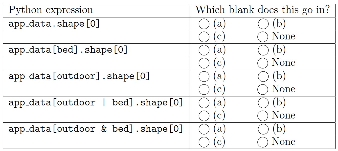
Answer: Reading the table from top to bottom, the five expressions should be used in the following blanks: None, (b), (a), (c), None.
The correct way to define obs_diff is
    outdoor = (app_data.get('category')=='outdoor')
    bed = (app_data.get('category')=='bed')
    obs_diff = (app_data[outdoor].shape[0] - app_data[bed].shape[0]) / app_data[outdoor | bed].shape[0]
The first provided line of code defines a boolean Series called
outdoor with a value of True corresponding to
each outdoor furniture item in app_data. Using this as the
condition in a query results in a DataFrame of outdoor furniture items,
and using .shape[0] on this DataFrame gives the number of
outdoor furniture items. So app_data[outdoor].shape[0]
represents the number of outdoor furniture items in
app_data. Similarly, app_data[bed].shape[0]
represents the number of beds in app_data. Likewise,
app_data[outdoor | bed].shape[0] represents the total
number of outdoor furniture items and beds in app_data.
Notice that we need to use an or condition (|) to
get a DataFrame that contains both outdoor furniture and beds.
We are told that the test statistic should be the proportion of outdoor furniture minus the proportion of beds. Translating this directly into code, this means the test statistic should be calculated as
obs_diff = app_data[outdoor].shape[0]/app_data[outdoor | bed].shape[0] - app_data[bed].shape[0]) / app_data[outdoor | bed].shape[0]Since this is a difference of two fractions with the same denominator, we can equivalently subtract the numerators first, then divide by the common denominator, using the mathematical fact \frac{a}{c} - \frac{b}{c} = \frac{a-b}{c}.
This yields the answer
obs_diff = (app_data[outdoor].shape[0] - app_data[bed].shape[0]) / app_data[outdoor | bed].shape[0]Notice that this is the observed value of the test statistic
because it’s based on the real-life data in the app_data
DataFrame, not simulated data.
The average score on this problem was 90%.
Which of the following is a valid way to generate one value of the test statistic according to the null model? Select all that apply.
Way 1:
multi = np.random.multinomial(2500, [0.5,0.5])
(multi[0] - multi[1])/2500
Way 2:
outdoor = np.random.multinomial(2500, [0.5,0.5])[0]/2500
bed = np.random.multinomial(2500, [0.5,0.5])[1]/2500
outdoor - bed
Way 3:
choice = np.random.choice([0, 1], 2500, replace=True)
choice_sum = choice.sum()
(choice_sum - (2500 - choice_sum))/2500
Way 4:
choice = np.random.choice(['bed', 'outdoor'], 2500, replace=True)
bed = np.count_nonzero(choice=='bed')
outdoor = np.count_nonzero(choice=='outdoor')
outdoor/2500 - bed/2500
Way 5:
outdoor = (app_data.get('category')=='outdoor')
bed = (app_data.get('category')=='bed')
samp = app_data[outdoor|bed].sample(2500, replace=True)
samp[samp.get('category')=='outdoor'].shape[0]/2500 -  samp[samp.get('category')=='bed'].shape[0]/2500)
Way 6:
outdoor = (app_data.get('category')=='outdoor')
bed = (app_data.get('category')=='bed')
samp = (app_data[outdoor|bed].groupby('category').count().reset_index().sample(2500, replace=True))
samp[samp.get('category')=='outdoor'].shape[0]/2500 - samp[samp.get('category')=='bed'].shape[0]/2500
Way 1
Way 2
Way 3
Way 4
Way 5
Way 6
Answer: Way 1, Way 3, Way 4, Way 6
Let’s consider each way in order.
Way 1 is a correct solution. This code begins by defining a variable
multi which will evaluate to an array with two elements
representing the number of items in each of the two categories, after
2500 items are drawn randomly from the two categories, with each
category being equally likely. In this case, our categories are beds and
outdoor furniture, and the null hypothesis says that each category is
equally likely, so this describes our scenario accurately. We can
interpret multi[0] as the number of outdoor furniture items
and multi[1] as the number of beds when we draw 2500 of
these items with equal probability. Using the same mathematical fact
from the solution to Problem 8.2, we can calculate the difference in
proportions as the difference in number divided by the total, so it is
correct to calculate the test statistic as
(multi[0] - multi[1])/2500.
Way 2 is an incorrect solution. Way 2 is based on a similar idea as
Way 1, except it calls np.random.multinomial twice, which
corresponds to two separate random processes of selecting 2500 items,
each of which is equally likely to be a bed or an outdoor furniture
item. However, is not guaranteed that the number of outdoor furniture
items in the first random selection plus the number of beds in the
second random selection totals 2500. Way 2 calculates the proportion of
outdoor furniture items in one random selection minus the proportion of
beds in another. What we want to do instead is calculate the difference
between the proportion of outdoor furniture and beds in a single random
draw.
Way 3 is a correct solution. Way 3 does the random selection of items
in a different way, using np.random.choice. Way 3 creates a
variable called choice which is an array of 2500 values.
Each value is chosen from the list [0,1] with each of the
two list elements being equally likely to be chosen. Of course, since we
are choosing 2500 items from a list of size 2, we must allow
replacements. We can interpret the elements of choice by
thinking of each 1 as an outdoor furniture item and each 0 as a bed. By
doing so, this random selection process matches up with the assumptions
of the null hypothesis. Then the sum of the elements of
choice represents the total number of outdoor furniture
items, which the code saves as the variable choice_sum.
Since there are 2500 beds and outdoor furniture items in total,
2500 - choice_sum represents the total number of beds.
Therefore, the test statistic here is correctly calculated as the number
of outdoor furniture items minus the number of beds, all divided by the
total number of items, which is 2500.
Way 4 is a correct solution. Way 4 is similar to Way 3, except
instead of using 0s and 1s, it uses the strings 'bed' and
'outdoor' in the choice array, so the
interpretation is even more direct. Another difference is the way the
number of beds and number of outdoor furniture items is calculated. It
uses np.count_nonzero instead of sum, which wouldn’t make
sense with strings. This solution calculates the proportion of outdoor
furniture minus the proportion of beds directly.
Way 5 is an incorrect solution. As described in the solution to
Problem 8.2, app_data[outdoor|bed] is a DataFrame
containing just the outdoor furniture items and the beds from
app_data. Based on the given information, we know
app_data[outdoor|bed] has 2500 rows, 1000 of which
correspond to beds and 1500 of which correspond to furniture items. This
code defines a variable samp that comes from sampling this
DataFrame 2500 times with replacement. This means that each row of
samp is equally likely to be any of the 2500 rows of
app_data[outdoor|bed]. The fraction of these rows that are
beds is 1000/2500 = 2/5 and the
fraction of these rows that are outdoor furniture items is 1500/2500 = 3/5. This means the random
process of selecting rows randomly such that each row is equally likely
does not make each item equally likely to be a bed or outdoor furniture
item. Therefore, this approach does not align with the assumptions of
the null hypothesis.
Way 6 is a correct solution. Way 6 essentially modifies Way 5 to make
beds and outdoor furniture items equally likely to be selected in the
random sample. As in Way 5, the code involves the DataFrame
app_data[outdoor|bed] which contains 1000 beds and 1500
outdoor furniture items. Then this DataFrame is grouped by
'category' which results in a DataFrame indexed by
'category', which will have only two rows, since there are
only two values of 'category', either
'outdoor' or 'bed'. The aggregation function
.count() is irrelevant here. When the index is reset,
'category' becomes a column. Now, randomly sampling from
this two-row grouped DataFrame such that each row is equally likely to
be selected does correspond to choosing items such that each
item is equally likely to be a bed or outdoor furniture item. The last
line simply calculates the proportion of outdoor furniture items minus
the proportion of beds in our random sample drawn according to the null
model.
The average score on this problem was 59%.
Suppose we generate 10,000 simulated values of the test statistic
according to the null model and store them in an array called
simulated_diffs. Complete the code below to calculate the
p-value for the hypothesis test.
np.count_nonzero(simulated_diffs _________ obs_diff)/10000What goes in the blank?
<
<=
>
>=
Answer: <=
To answer this question, we need to know whether small values or large values of the test statistic indicate the alternative hypothesis. The alternative hypothesis is that IKEA sells more beds than outdoor furniture. Since we’re calculating the proportion of outdoor furniture minus the proportion of beds, this difference will be small (negative) if the alternative hypothesis is true. Larger (positive) values of the test statistic mean that IKEA sells more outdoor furniture than beds. A value near 0 means they sell beds and outdoor furniture equally.
The p-value is defined as the proportion of simulated test statistics
that are equal to the observed value or more extreme, where extreme
means in the direction of the alternative. In this case, since small
values of the test statistic indicate the alternative hypothesis, the
correct answer is <=.
The average score on this problem was 43%.
In some cities, the number of sunshine hours per month is relatively consistent throughout the year. São Paulo, Brazil is one such city; in all months of the year, the number of sunshine hours per month is somewhere between 139 and 173. New York City’s, on the other hand, ranges from 139 to 268.
Gina and Abel, both San Diego natives, are interested in assessing how “consistent" the number of sunshine hours per month in San Diego appear to be. Specifically, they’d like to test the following hypotheses:
Null Hypothesis: The number of sunshine hours per month in San Diego is drawn from the uniform distribution, \left[\frac{1}{12}, \frac{1}{12}, ..., \frac{1}{12}\right]. (In other words, the number of sunshine hours per month in San Diego is equal in all 12 months of the year.)
Alternative Hypothesis: The number of sunshine hours per month in San Diego is not drawn from the uniform distribution.
As their test statistic, Gina and Abel choose the total variation distance. To simulate samples under the null, they will sample from a categorical distribution with 12 categories — January, February, and so on, through December — each of which have an equal probability of being chosen.
In order to run their hypothesis test, Gina and Abel need a way to calculate their test statistic. Below is an incomplete implementation of a function that computes the TVD between two arrays of length 12, each of which represent a categorical distribution.
    def calculate_tvd(dist1, dist2):
        return np.mean(np.abs(dist1 - dist2)) * ____
Fill in the blank so that calculate_tvd works as
intended.
1 / 6
1 / 3
1 / 2
2
3
6
Answer: 6
The TVD is the sum of the absolute differences in proportions,
divided by 2. In the code to the left of the blank, we’ve computed the
mean of the absolute differences in proportions, which is the same as
the sum of the absolute differences in proportions, divided by 12 (since
len(dist1) is 12). To correct the fact that we
divided by 12, we multiply by 6, so that we’re only dividing by 2.
The average score on this problem was 17%.
Moving forward, assume that calculate_tvd works
correctly.
Now, complete the implementation of the function
uniform_test, which takes in an array
observed_counts of length 12 containing the number of
sunshine hours each month in a city and returns the p-value for the
hypothesis test stated at the start of the question.
    def uniform_test(observed_counts):
        # The values in observed_counts are counts, not proportions!
        total_count = observed_counts.sum()
        uniform_dist = __(b)__
        tvds = np.array([])
        for i in np.arange(10000):
            simulated = __(c)__
            tvd = calculate_tvd(simulated, __(d)__)
            tvds = np.append(tvds, tvd)
return np.mean(tvds __(e)__ calculate_tvd(uniform_dist, __(f)__))What goes in blank (b)? (Hint: The function
np.ones(k) returns an array of length k in
which all elements are 1.)
Answer: np.ones(12) / 12
uniform_dist needs to be the same as the uniform
distribution provided in the null hypothesis, \left[\frac{1}{12}, \frac{1}{12}, ...,
\frac{1}{12}\right].
In code, this is an array of length 12 in which each element is equal
to 1 / 12. np.ones(12)
creates an array of length 12 in which each value is 1; for
each value to be 1 / 12, we divide np.ones(12)
by 12.
The average score on this problem was 66%.
What goes in blank (c)?
np.random.multinomial(12, uniform_dist)
np.random.multinomial(12, uniform_dist) / 12
np.random.multinomial(12, uniform_dist) / total_count
np.random.multinomial(total_count, uniform_dist)
np.random.multinomial(total_count, uniform_dist) / 12
np.random.multinomial(total_count, uniform_dist) / total_count
Answer:
np.random.multinomial(total_count, uniform_dist) / total_count
The idea here is to repeatedly generate an array of proportions that
results from distributing total_count hours across the 12
months in a way that each month is equally likely to be chosen. Each
time we generate such an array, we’ll determine its TVD from the uniform
distribution; doing this repeatedly gives us an empirical distribution
of the TVD under the assumption the null hypothesis is true.
The average score on this problem was 21%.
What goes in blank (d)?
Answer: uniform_dist
As mentioned above:
Each time we generate such an array, we’ll determine its TVD from the uniform distribution; doing this repeatedly gives us an empirical distribution of the TVD under the assumption the null hypothesis is true.
The average score on this problem was 54%.
What goes in blank (e)?
>
>=
<
<=
==
!=
Answer: >=
The purpose of the last line of code is to compute the p-value for the hypothesis test. Recall, the p-value of a hypothesis test is the proportion of simulated test statistics that are as or more extreme than the observed test statistic, under the assumption the null hypothesis is true. In this context, “as extreme or more extreme” means the simulated TVD is greater than or equal to the observed TVD (since larger TVDs mean “more different”).
The average score on this problem was 77%.
What goes in blank (f)?
Answer: observed_counts / total_count
or observed_counts / observed_counts.sum()
Blank (f) needs to contain the observed distribution of sunshine hours (as an array of proportions) that we compare against the uniform distribution to calculate the observed TVD. This observed TVD is then compared with the distribution of simulated TVDs to calculate the p-value. The observed counts are converted to proportions by dividing by the total count so that the observed distribution is on the same scale as the simulated and expected uniform distributions, which are also in proportions.
The average score on this problem was 27%.
Costin, a San Francisco native, will be back in San Francisco over the summer, and is curious as to whether it is true that about \frac{3}{4} of days in San Francisco are sunny.
Fast forward to the end of September: Costin counted that of the 30 days in September, 27 were sunny in San Francisco. To test his theory, Costin came up with two pairs of hypotheses.
Pair 1:
Null Hypothesis: The probability that it is sunny on any given day in September in San Francisco is \frac{3}{4}, independent of all other days.
Alternative Hypothesis: The probability that it is sunny on any given day in September in San Francisco is not \frac{3}{4}.
Pair 2:
Null Hypothesis: The probability that it is sunny on any given day in September in San Francisco is \frac{3}{4}, independent of all other days.
Alternative Hypothesis: The probability that it is sunny on any given day in September in San Francisco is greater than \frac{3}{4}.
For each test statistic below, choose whether the test statistic could be used to test Pair 1, Pair 2, both, or neither. Assume that all days are either sunny or cloudy, and that we cannot perform two-tailed hypothesis tests. (If you don’t know what those are, you don’t need to!)
The difference between the number of sunny days and number of cloudy days
Pair 1
Pair 2
Both
Neither
Answer: Pair 2
The test statistic provided is the difference between the number of sunny days and cloudy days in a sample of 30 days. Since each day is either sunny or cloudy, the number of cloudy days is just 30 - the number of sunny days. This means we can re-write our test statistic as follows:
\begin{align*} &\text{number of sunny days} - \text{number of cloudy days} \\ &= \text{number of sunny days} - (30 - \text{number of sunny days}) \\ &= 2 \cdot \text{number of sunny days} - 30 \\ &= 2 \cdot (\text{number of sunny days} - 15) \end{align*}
The more sunny days there are in our sample of 30 days, the larger this test statistic will be. (Specifically, if there are more sunny days than cloudy days, this will be positive; if there’s an equal number of sunny and cloudy days, this will be 0, and if there are more cloudy days, this will be negative.)
Now, let’s look at each pair of hypotheses.
Pair 1:
Pair 1’s alternative hypothesis is that the probability of a sunny day is not \frac{3}{4}, which includes both greater than and less than \frac{3}{4}.
To test this pair of hypotheses, we need a test statistic that is large when the number of sunny days is far from \frac{3}{4} (evidence for the alternative hypothesis) and small when the number of sunny days is close to \frac{3}{4} (evidence for the null hypothesis). (It would also be acceptable to design a test statistic that is small when the number of sunny days is far from \frac{3}{4} and large when it’s close to \frac{3}{4}, but the first option we’ve outlined is a bit more natural.)
Our chosen test statistic, 2 \cdot (\text{number of sunny days} - 15), doesn’t work this way; both very large values and very small values indicate that the proportion of sunny days is far from \frac{3}{4}, and since we can’t use two-tailed tests, we can’t use our test statistic for this pair.
Pair 2:
Pair 2’s alternative hypothesis is that the probability of a sunny day greater than \frac{3}{4}.
Since our test statistic is large when the number of sunny days is large (evidence for the alternative hypothesis) and is small when the number of sunny days is small (evidence for the null hypothesis), we can use our test statistic to test this pair of hypotheses. The key difference between Pair 1 and Pair 2 is that Pair 2’s alternative hypothesis has a direction – it says that the probability that it is sunny on any given day is greater than \frac{3}{4}, rather than just “not” \frac{3}{4}.
Thus, we can use this test statistic to test Pair 2, but not Pair 1.
The average score on this problem was 28%.
The absolute difference between the number of sunny days and number of cloudy days
Pair 1
Pair 2
Both
Neither
Answer: Neither
The test statistic here is the absolute value of the test statistic in the first part. Since we were able to re-write the test statistic in the first part as 2 \cdot (\text{number of sunny days} - 15), our test statistic here is |2 \cdot (\text{number of sunny days} - 15)|, or, since 2 already non-negative,
2 \cdot | \text{number of sunny days} - 15 |
This test statistic is large when the number of sunny days is far from 15, i.e. when the number of sunny days and number of cloudy days are far apart, or when the proportion of sunny days is far from \frac{1}{2}. However, the null hypothesis we’re testing here is not that the proportion of sunny days is \frac{1}{2}, but that the proportion of sunny days is \frac{3}{4}.
A large value of this test statistic will tell us the proportion of sunny days is far from \frac{1}{2}, but it may or may not be far from \frac{3}{4}. For instance, when \text{number of sunny days} = 7, then our test statistic is 2 \cdot | 7 - 15 | = 16. When \text{number of sunny days} = 23, our test statistic is also 16. However, in the first case, the proportion of sunny days is just under \frac{1}{4} (far from \frac{3}{4}), while in the second case the proportion of sunny days is just above \frac{3}{4}.
In both pairs of hypotheses, this test statistic isn’t set up such that large values point to one hypothesis and small values point to the other, so it can’t be used to test either pair.
The average score on this problem was 25%.
The difference between the proportion of sunny days and \frac{1}{4}
Pair 1
Pair 2
Both
Neither
Answer: Pair 2
The test statistic here is the difference between the proportion of sunny days and \frac{1}{4}. This means if p is the proportion of sunny days, the test statistic is p - \frac{1}{4}. This test statistic is large when the proportion of sunny days is large and small when the proportion of sunny days is small. (The fact that we’re subtracting by \frac{1}{4} doesn’t change this pattern – all it does is shift both the empirical distribution of the test statistic and our observed statistic \frac{1}{4} of a unit to the left on the x-axis.)
As such, this test statistic behaves the same as the test statistic from the first part – both test statistics are large when the number of sunny days is large (evidence for the alternative hypothesis) and small when the number of sunny days is small (evidence for the null hypothesis). This means that, like in the first part, we can use this test statistic to test Pair 2, but not Pair 1.
The average score on this problem was 24%.
The absolute difference between the proportion of cloudy days and \frac{1}{4}
Pair 1
Pair 2
Both
Neither
Answer: Pair 1
The test statistic here is the absolute difference between the proportion of cloudy days and \frac{1}{4}. Let q be the proportion of cloudy days. The test statistic is |q - \frac{1}{4}|. The null hypothesis for both pairs states that the probability of a sunny day is \frac{3}{4}, which implies the probability of a cloudy day is \frac{1}{4} (since all days are either sunny or cloudy).
This test statistic is large when the proportion of cloudy days is far from \frac{1}{4} and small when the proportion of cloudy days is close to \frac{1}{4}.
Since Pair 1’s alternative hypothesis is just that the proportion of cloudy days is not \frac{1}{4}, we can use this test statistic to test it! Large values of this test statistic point to the alternative hypothesis and small values point to the null.
On the other hand, Pair 2’s alternative hypothesis is that the proportion of sunny days is greater than \frac{3}{4}, which is the same as the proportion of cloudy days being less than \frac{1}{4}. The issue here is that our test statistic doesn’t involve a direction – a large value implies that the proportion of cloudy days is far from \frac{1}{4}, but we don’t know if that means that there were fewer cloudy days than \frac{1}{4} (evidence for Pair 2’s alternative hypothesis) or more cloudy days than \frac{1}{4} (evidence for Pair 2’s null hypothesis). Since, for Pair 2, this test statistic isn’t set up such that large values point to one hypothesis and small values point to the other, we can’t use this test statistic to test Pair 2.
Therefore, we can use this test statistic to test Pair 1, but not Pair 2.
Aside: This test statistic is equivalent to the absolute difference between the proportion of sunny days and \frac{3}{4}. Try and prove this fact!
The average score on this problem was 46%.
The table below shows the proportion of apartments of each type in each of three neighborhoods. Note that each column sums to 1.
| Type | North Park | Chula Vista | La Jolla |
|---|---|---|---|
| Studio | 0.30 | 0.15 | 0.40 |
| One bedroom | 0.40 | 0.35 | 0.30 |
| Two bedroom | 0.20 | 0.25 | 0.15 |
| Three bedroom | 0.10 | 0.25 | 0.15 |
Find the total variation distance (TVD) between North Park and Chula Vista. Give your answer as an exact decimal.
Answer: 0.2
To find the TVD, we take the absolute differences between North Park and Chula Vista for all rows, sum them, then cut the result in half.
\dfrac{|0.3 - 0.15| + |0.4 - 0.35| + |0.2 - 0.25| + |0.1 - 0.25|}{2} = \dfrac{0.15 + 0.05 + 0.05 + 0.15}{2} = \dfrac{0.4}{2} = 0.2
The average score on this problem was 72%.
Which pair of neighborhoods is most similar in terms of types of housing, as measured by TVD?
North Park and Chula Vista
North Park and La Jolla
Chula Vista and La Jolla
Answer: North Park and La Jolla
The TVD between North Park and La Jolla is the lowest between all pairs of two of these three neighborhoods:
| Pair | TVD |
|---|---|
| North Park and Chula Vista | 0.2 |
| North Park and La Jolla | 0.15 |
| Chula Vista and La Jolla | 0.25 |
This implies that the distributions of apartment types for North Park and La Jolla are the most similar.
The average score on this problem was 94%.
25% of apartments in Little Italy are one bedroom apartments. Based on this information, what is the minimum and maximum possible TVD between North Park and Little Italy? Give your answers as exact decimals.
Answer:
The minimum TVD is 0.15 because:
The maximum TVD is 0.65 because:
The average score on this problem was 49%.
The average score on this problem was 33%.
[(13 pts)]
In certain districts (1, 2, and 4), children spend years training for the Hunger Games and frequently volunteer to participate in them. Tributes that come from these districts are known as Career tributes. Many residents of Panem believe that Career tributes generally fare better in the Hunger Games because of their extensive training.
We’ll test this claim using historical data. The DataFrame
survival has a row for each tribute who participated in one
of the first 74 Hunger Games. The
columns are as follows:
"Tribute": The name of the tribute.
"District": Their home district (1–12).
"Days": The number of days they stayed alive in the
arena.
"Game": The Hunger Games edition they competed in
(1–74).
A few rows of survival are shown below:

We’ll use this data to test the following pair of hypotheses:
Null Hypothesis: On average, Career tributes and
non-Career tributes survive an equal amount of time in the arena.
Alternative Hypothesis: On average, Career tributes survive longer in the arena than non-Career tributes.
Our test statistic will be the mean survival time of Career tributes minus the mean survival time of non-Career tributes
Write code to create a DataFrame called tributes that
has all the data in survival plus an additional column
called "Career". This column should contain boolean values
indicating whether each tribute is considered a Career tribute. Feel
free to define intermediate variables and functions as needed, and to do
this in multiple lines of code.
Answer:
def is_career(d):
    if d==1 or d==2 or d==4:
        return True
    else:
        return False
tributes = survival.assign(Career=survival.get('District').apply(is_career))
A quick explaination here would be saying that inorder to have a new column where we can decipher if a given tribute is a career tribute or not, we need a function that tells us if a tribute is a career tribute based on the district they are located in. To do this, all we need to do is check for any given tribute if they are in districts 1, 2, or 4 using our function, meaning we need to build our function and then apply it to the district series. We can then just assign the output series back to the original dataframe.
The average score on this problem was 65%.
Fill in the blanks in the code below so that statistics
evaluates to an array with 10000 simulated values of the test statistic
under the null hypothesis.
statistics = np.array([])

for i in np.arange(10000):
    shuffled = tributes.assign(__(a)__)
    means = shuffled.groupby("Career").mean().get("Days")
    stat = __(b)__
statistics = np.append(statistics, stat)Answer:
(a):
Days = np.random.permutation(tributes.get("Days")) OR
Career = np.random.permutation(tributes.get("Career"))
(b): means.loc[True] - means.loc[False]
In blank a we shuffle one of the columns so as to break any real link
between the Career column and the Days column. This allows us to
simulate our null hypothesis. After this in blank b, we use
means.loc[True] - means.loc[False] to get the difference in
mean survival days between career and non-career tributes. This is our
test statistic.
The average score on this problem was 63%.
The output of tributes.groupby("Career").mean() is shown
below.
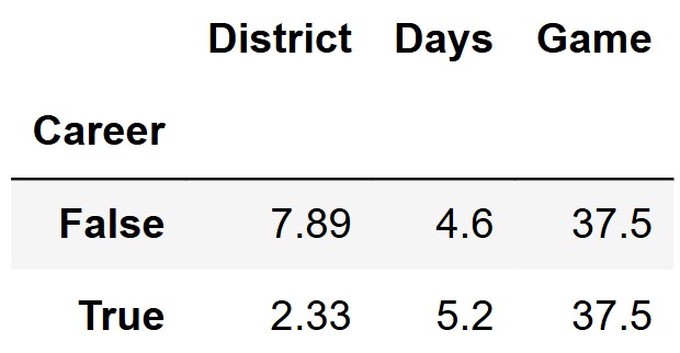
Fill in the blank below to compute the p-value of this test.
p_value = (__(a)__).mean()Answer:
(a): statistics >= 0.6
Our observed statistic can be calculated by taking the difference in
means from the Days column. In this case that is 5.2 - 4.6 = 0.6. We want all of the simulated
values that are at least as extreme as this observed value. Therefore we
want all values from the statistics array >= 0.6.
The average score on this problem was 63%.
You want to test the following hypotheses:
Null Hypothesis: Everyone who applies for an internship at Google has a 20% chance of receiving a job offer, independently of all other applicants.
Alternative Hypothesis: Everyone who applies for an internship at Google has a more than 20% chance of receiving a job offer, independently of all other applicants.
To test these hypotheses, you collected information from 50 applicants and found that 16 of them received a job offer.
Fill in the blanks in the code below to calculate the p-value for a hypothesis test where the test statistic is the number of applicants, out of 50, who receive a job offer.
offers_array = np.array([])

for i in np.arange(10000):
    num_offers = ___(a)___
    offers_array = ___(b)___

p_value = ___(c)___
p_valueAnswer:
(a):
np.random.multinomial(50,[0.2,0.8])[0] or np.random.choice([0,1], 50, p = [0.80, 0.20]).sum()
(b): np.append(offers_array, num_offers)
(c):
np.count_nonzero(offers_array >= 16)/10000 or np.mean(offers_array >= 16)
The average score on this problem was 70%.
Suppose the p-value comes out to 0.03. What conclusion do we draw?
We reject the null hypothesis at both the 0.01 and 0.05
We fail to reject the null hypothesis at the 0.01 significance
We reject the null hypothesis at the 0.01 significance level and
We fail to reject the null hypothesis at both the 0.01 and 0.05
Answer: Option 2
The average score on this problem was 62%.
Which of the following test statistics would have also been appropriate to test these hypotheses? Select all that apply.
Number of applicants, out of 50, who do not receive a job offer.
Proportion of applicants that receive a job offer.
The sum of the absolute differences between [0.2, 0.8] and the
Absolute difference between 20 and the number of applicants, out
None of the above.
Answer: Options 1 and 2
The average score on this problem was 68%.
Every year, the American Kennel Club holds a Photo Contest for dogs. Eric wants to know whether toy dogs win disproportionately more often than other kinds of dogs. He has collected a sample of 500 dogs that have won the Photo Contest. In his sample, 200 dogs were toy dogs.
Eric also knows the distribution of dog kinds in the population:
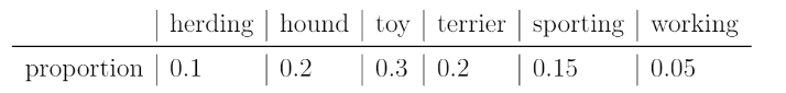
Select all correct statements of the null hypothesis.
The distribution of dogs in the sample is the same as the distribution in the population. Any difference is due to chance.
Every dog in the sample was drawn uniformly at random without replacement from the population.
The number of toy dogs that win is the same as the number of toy dogs in the population.
The proportion of toy dogs that win is the same as the proportion of toy dogs in the population.
The proportion of toy dogs that win is 0.3.
The proportion of toy dogs that win is 0.5.
Answer: Options 4 & 5
A null hypothesis is the hypothesis that there is no significant difference between specified populations, any observed difference being due to sampling or experimental error. Let’s consider what a potential null hypothesis might look like. A potential null hypothesis would be that there is no difference between the win proportion of toy dogs compared to the proportion of toy dogs in the population.
Option 1: We’re not really looking at the distribution of dogs in our sample vs. dogs in our population, rather, we’re looking at whether toy dogs win more than other dogs. In other words, the only factors we’re really consdiering are the proportion of toy dogs to normal dogs, as well as the win percentages of toy dogs to normal dogs; and so the distribution of the population doesn’t really matter. Furthermore, this option makes no reference to win rate of toy dogs.
Option 2: This isn’t really even a null hypothesis, but rather more of a description of a test procedure. This option also makes no attempt to reference to win rate of toy dogs.
Option 3: This statement doesn’t really make sense in that it is illogical to compare the raw number of toy dogs wins to the number of toy dogs in the population, because the number of toy dogs is always at least the number of toy dogs that win.
Option 4: This statement is in line with the null hypothesis.
Option 5: This statement is another potential null hypothesis since the proportion of toy dogs in the population is 0.3.
Option 6: This statement, although similar to Option 5, would not be a null hypothesis because 0.5 has no relevance to any of the relevant proportions. While it’s true that if the proportion of of toy dogs that win is over 0.5, we could maybe infer that toy dogs win the majority of the times; however, the question is not to determine whether toy dogs win most of the times, but rather if toy dogs win a disproportionately high number of times relative to its population size.
The average score on this problem was 83%.
Select the correct statement of the alternative hypothesis.
The model in the null hypothesis underestimates how often toy dogs win.
The model in the null hypothesis overestimates how often toy dogs win.
The distribution of dog kinds in the sample is not the same as the population.
The data were not drawn at random from the population.
Answer: Option 1
The alternative hypothesis is the hypothesis we’re trying to support, which in this case is that toy dogs happen to win more than other dogs.
Option 1: This is in line with our alternative hypothesis, since proving that the null hypothesis underestimates how often toy dogs win means that toy dogs win more than other dogs.
Option 2: This is the opposite of what we’re trying to prove.
Option 3: We don’t really care too much about the distribution of dog kinds, since that doesn’t help us determine toy dog win rates compared to other dogs.
Option 4: Again, we don’t care whether all dogs are chosen according to the probabilities in the null model, instead we care specifically about toy dogs.
The average score on this problem was 67%.
Select all the test statistics that Eric can use to conduct his hypothesis.
The proportion of toy dogs in his sample.
The number of toy dogs in his sample.
The absolute difference of the sample proportion of toy dogs and 0.3.
The absolute difference of the sample proportion of toy dogs and 0.5.
The TVD between his sample and the population.
Answer: Option 1 and Option 2
Option 1: This option is correct. According to our null hypothesis, we’re trying to compare the proportion of toy dogs win rates to the proportion of toy dogs. Thus taking the proportion of toy dogs in Eric’s sample is a perfectly valid test statistic.
Option 2: This option is correct. Since the sample size is fixed at 500, so kowning the count is equivalent to knowing the proportion.
Option 3: This option is incorrect. The absolute difference of the sample proportion of toy dogs and 0.3 doesn’t help us because the absolute difference won’t tell us whether or not the sample proportion of toy dogs is lower than 0.3 or higher than 0.3.
Option 4: This option is incorrect for the same reasoning as above, but also 0.5 isn’t a relevant number anyways.
Option 5: This option is incorrect because TVD measures distance between two categorical distributions, and here we only care about one particular category (not all categories) being the same.
The average score on this problem was 70%.
Eric decides on this test statistic: the proportion of toy dogs minus the proportion of non-toy dogs. What is the observed value of the test statistic?
-0.4
-0.2
0
0.2
0.4
Answer: -0.2
For our given sample, the proportion of toy dogs is \frac{200}{500}=0.4 and the proportion of non-toy dogs is \frac{500-200}{500}=0.6, so 0.4 - 0.6 = -0.2.
The average score on this problem was 74%.
Which snippets of code correctly compute Eric’s test statistic on one
simulated sample under the null hypothesis? Select all that apply. The
result must be stored in the variable stat. Below are the 5
snippets
Snippet 1:
a = np.random.choice([0.3, 0.7])
b = np.random.choice([0.3, 0.7])
stat = a - b
Snippet 2:
a = np.random.choice([0.1, 0.2, 0.3, 0.2, 0.15, 0.05])
stat = a - (1 - a)
Snippet 3:
a = np.random.multinomial(500, [0.1, 0.2, 0.3, 0.2, 0.15, 0.05]) / 500
stat = a[2] - (1 - a[2])
Snippet 4:
a = np.random.multinomial(500, [0.3, 0.7]) / 500
stat = a[0] - (1 - a[0])
Snippet 5:
a = df.sample(500, replace=True)
b = a[a.get("kind") == "toy"].shape[0] / 500
stat = b - (1 - b)
Snippet 1
Snippet 2
Snippet 3
Snippet 4
Snippet 5
Answer: Snippet 3 & Snippet 4
Snippet 1: This is incorrect because
np.random.choice() only chooses values that are either 0.3
or 0.7 which is simply just wrong.
Snippet 2: This is wrong because np.random.choice()
only chooses from the values within the list. From a sanity check it’s
not hard to realize that a should be able to take on more
values than the ones in the list.
Snippet 3: This option is correct. Recall, in
np.random.multinomial(n, [p_1, ..., p_k]), n
is the number of experiments, and [p_1, ..., p_k] is a
sequence of probability. The method returns an array of length k in
which each element contains the number of occurrences of an event, where
the probability of the ith event is p_i. In this snippet,
np.random.multinomial(500, [0.1, 0.2, 0.3, 0.2, 0.15, 0.05])
generates a array of length 6
(len([0.1, 0.2, 0.3, 0.2, 0.15, 0.05])) that contains the
number of occurrences of each kinds of dogs according to the given
distribution (the population distribution). We divide the first line by
500 to convert the number of counts in our resulting array into
proportions. To access the proportion of toy dogs in our sample, we take
the entry with the probability ditribution value of 0.3, which is the
third entry in the array or a[2]. To calculate our test
statistic we take the proportion of toy dogs minus the proportion of
non-toy dogs or a[2] - (1 - a[2])
Snippet 4: This option is correct. This approach is similar to the one above except we’re only considering the probability distribution of toy dogs vs non-toy dogs, which is what we wanted in the first place. The rest of the steps are similar to the ones above.
Snippet 5: Note that df is simple just a dataframe
containing information of the dogs, and may or may not reflect the
population distribution of dogs that participate in the photo
contest.
The average score on this problem was 72%.
After simulating, Eric has an array called sim that
stores his simulated test statistics, and a variable called
obs that stores his observed test statistic.
What should go in the blank to compute the p-value?
np.mean(sim _______ obs) <
<=
==
>=
>
Answer: Option 4: >=
Note that to calculate the p-value we look for test statistics that
are equal to the observed statistic or even further in the direction of
the alternative. In this case, if the proportion of the population of
toy dogs compared to the rest of the dog population was higher than
observed, we’d get a value larger than 0.2, and thus we use
>=.
The average score on this problem was 66%.
Eric’s p-value is 0.03. If his p-value cutoff is 0.01, what does he conclude?
He rejects the null in favor of the alternative.
He accepts the null.
He accepts the aleternative.
He fails to reject the null.
Answer: Option 4: He fails to reject the null
Option 1: Note that since our p-value was greater than 0.01, we fail to reject the null.
Option 2: We can never “accept” the null hypothesis.
Option 3: We didn’t accept the alternative since we failed to reject the null.
Option 4: This option is correct because our p-value was larger than our cutoff.
The average score on this problem was 86%.
You are analyzing the data in stages to see which
countries winners come from.
You categorize the countries into four groups: France, Italy, Belgium, and Other. After performing some analysis, you find that the observed distribution of countries of origin for Tour de France stage winners is [0.3, 0.2, 0.1, 0.4]; i.e. 30% of stage winners are French, 20% Italian, etc. Based on census information, the expected population distribution is [0.07, 0.06, 0.01, 0.86]; that is, France’s total population is 7% of the sum of the populations of all countries participating in the Tour, Italy’s is 6%, etc.
You conduct a hypothesis test with the following hypotheses:
Which of the following test statistics are appropriate for this hypothesis test? Select all that apply.
The absolute difference between the expected proportion of French stage winners and the observed proportion of French stage winners.
The sum of the differences between the expected population distribution and the observed distribution of stage winners.
The absolute difference between the number of French stage winners and the number of Italian stage winners.
The sum of the absolute differences between the expected population distribution and the observed distribution of stage winners.
Answer: Option 1 and Option 4
The average score on this problem was 80%.
For the rest of this question, assume that we will be using the Total Variation Distance as our test statistic.
Complete the implementation of the simulate and
calculate_test_stat functions so that the code below
successfully simulates 10,000 test statistics.
expected_dist = [0.07, 0.06, 0.01, 0.86]
observed_dist = [0.3, 0.2, 0.1, 0.4]

def simulate(__(i)__):
    simulated_winners = np.random.__(ii)__(100, __(iii)__)
    return simulated_winners / 100

def calculate_test_stat(__(iv)__, __(v)__):
    return __(vi)__


observed_stat = calculate_test_stat(observed_dist, expected_dist)
simulated_stats = np.array([])
for i in np.arange(10000):
    simulated_dist = simulate(expected_dist)
    simulated_stat = calculate_test_stat(simulated_dist, expected_dist)
simulated_stats = np.append(simulated_stats, simulated_stat)Answer:
expected_distmultinomialexpected_distsimulated_distexpected_dist (or swapped with
above)np.abs(simulated dist - expected dist).sum() / 2When performing a simulation, we simulated based on the expectation.
Thus, the argument for the simulate function (i) should
be the expected_dist array.
In this function, we simulate winners based on the expected
distribution. So, we want to use np.random.multinomial in
(ii) which will take in the number of experiments and
expected distribution, ie expected_dist in
(iii), which is an array of the probabilities for each
of the outcomes.
We are using the total variation distance as the test statistic. The
Total Variation Distance (TVD) of two categorical distributions is the
sum of the absolute differences of their proportions, all divided by 2.
Thus, the arguments of the calculate_test_stat function
should be the simulated_distribution in
(iv) and the expected_distribution in
(v) (or swapped).
In this function, we need to return the TVD which can be calculated
as follows:
np.abs(simulated dist - expected dist).sum() / 2 in
(vi).
The average score on this problem was 89%.
Fill in the blank in the following code so that p_value
evaluates to the correct p-value for this hypothesis test:
p_value = np.mean(simulated_stats ___ observed_statistic)>
>=
<
<=
=
Answer: >=
Recall the p-value is the probability of seeing a result equal to or more extreme than the observed value under the null hypothesis. Since the TVD is our test statistic where greater values indicate a result more extreme that means we want to use >= in the blank to check whether the simulated statistic is equal to or more extreme than the observed statistic.
The average score on this problem was 80%.
ESPN (a large sports news network) states that the Las Vegas Aces have a 60% chance of winning their upcoming game. You’re curious as to how they came up with this estimate, and you decide to conduct a hypothesis test for the following hypotheses:
Null Hypothesis: The Las Vegas Aces win each game with a probability of 60%.
Alternative Hypothesis: The Las Vegas Aces win each game with a probability above 60%.
In both hypotheses, we are assuming that each game is independent of all other games.
In the 2021 season, the Las Vegas Aces won 22 of their games and lost 9 of their games.
Below, we have provided the code necessary to conduct the hypothesis test described above.
stats = np.array([])
for i in np.arange(10000):
    sim = np.random.multinomial(31, [0.6, 0.4])
    stat = fn(sim)
    stats = np.append(stats, stat)
win_p_value = np.count_nonzero(stats >= fn([22, 9])) / 10000
fn is a function that computes a test
statistic, given a list or array arr of two elements (the
first of which is the number of wins, and the second of which is the
number of losses). You can assume that neither element of
arr is equal to 0.
Below, we define 5 possible test statistics fn.
Option 1:
def fn(arr):
    return arr[0] / arr[1]
Option 2:
def fn(arr):
    return arr[0]
Option 3:
def fn(arr):
    return np.abs(arr[0] - arr[1])
Option 4:
def fn(arr):
    return arr[0] - arr[1]
Option 5:
def fn(arr):
    return arr[1] - arr[0]
Which of the above functions fn would be valid test
statistics for this hypothesis test and p-value calculation?
Select all that apply.
Option 1
Option 2
Option 3
Option 4
Option 5
Answer: Options 1, 2, and 4
In the code provided to us, stats is an array containing
10,000 p-values generated by the function fn (note that we
are appending stat to stats, and in the line
before that we have stat = fn(sim)). In the very last line
of the code provided, we have:
win_p_value = np.count_nonzero(stats >= fn([22, 9])) / 10000If we look closely, we see that we are computing the p-value by
computing the proportion of simulated test statistics that were
greater than or equal to (>=) the observed
statistic. Since a p-value is computed as the proportion of
simulated test statistics that were as or more extreme than the
observed statistic, here it must mean that “big” test
statistics are more extreme.
Remember, the direction that is “extreme” is determined by our
alternative hypothesis. Here, the alternative hypothesis is that the Las
Vegas Aces win each game with a probability above 60%. As such, the test
statistic(s) we choose must be large when the probability that
the Aces win a game is high, and small when the probability
that the Aces win a game is low. With this all in mind, we can take a
look at the 5 options, remembering that arr[0] is
the number of simulated wins and arr[1] is the number of
simulated losses in a season of 31 games. This means that when
the Aces win more than they lose, arr[0] > arr[1], and
when they lose more than they win, arr[0] < arr[1].
arr[0] / arr[1]. If the Aces win a
lot, the numerator will be larger than the denominator, so this ratio
will be large. If the Aces lose a lot, the numerator will be smaller
than the denominator, and so this ratio will be small. This is what we
want!arr[0]. If the Aces win a lot, this number will
be large, and if the Aces lose a lot, this number will be small. This is
what we want!np.abs(arr[0] - arr[1]). If the Aces win a lot, then
arr[0] - arr[1] will be large, and so will
np.abs(arr[0] - arr[1]). This seems fine.
However, if the Aces lose a lot, then
arr[0] - arr[1] will be small (negative), but
np.abs(arr[0] - arr[1]) will still be large and positive.
This test statistic doesn’t allow us to differentiate
when the Aces win a lot or lose a lot, so we can’t use it as a test
statistic for our alternative hypothesis.arr[0] - arr[1] is large.
Furthermore, when the Aces lose a lot, arr[0] - arr[1] is
small (negative numbers are small in this context). This works!arr[1] - arr[0] is the
opposite of arr[0] - arr[1] in Option 4. When the Aces win
a lot, arr[1] - arr[0] is small (negative), and when the
Aces lose a lot, arr[1] - arr[0] is large (positive). This
is the opposite of what we want, so Option 5 does not work.
The average score on this problem was 77%.
The empirical distribution of one of the 5 test statistics presented
in the previous subpart is shown below. To draw the histogram, we used
the argument bins=np.arange(-10, 25).
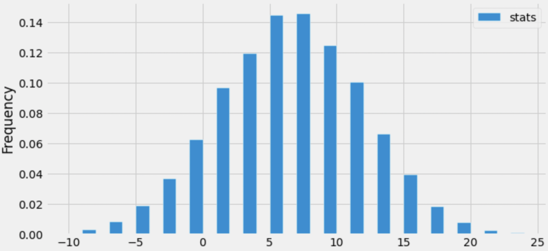
Which test statistic does the above empirical distribution belong to?
Option 1
Option 2
Option 3
Option 4
Option 5
Answer: Option 4
The distribution visualized in the histogram has the following unique values: -9, -7, -5, -3, …, 17, 19, 21, 23. Crucially, the test statistic whose distribution we’ve visualized can both be positive and negative. Right off the bat, we can eliminate Options 1, 2, and 3:
arr[0]) by the number of losses
(arr[1]), and that quotient will always be a non-negative
number.arr[0]) will always be a non-negative number.np.abs(arr[0] - arr[1]), in this case) will
always be a non-negative number.Now, we must decide between Option 4, whose test statistic is “wins
minus losses” (arr[0] - arr[1]), and Option 5, whose test
statistic is “losses minus wins” (arr[1] - arr[0]).
First, let’s recap how we’re simulating. In the code
provided in the previous subpart, we have the line
sim = np.random.multinomial(31, [0.6, 0.4]). Each time we
run this line, sim will be set to an array with two
elements, the first of which we interpret as the number of simulated
wins and the second of which we interpret as the number of simulated
losses in a 31 game season. The first number in sim will
usually be larger than the second number in sim, since the
chance of a win (0.6) is larger than the chance of a loss (0.4). As
such, When we compute fn(sim) in the following line, the
difference between the wins and losses should typically be positive.
Back to our distribution. Note that the distribution provided in this subpart is centered at a positive number, around 7. Since the difference between wins and losses will typically be positive, it appears that we’ve visualized the distribution of the difference between wins and losses (Option 4). If we instead visualized the difference between losses and wins, the distribution should be centered at a negative number, but that’s not the case.
As such, the correct answer is Option 4.
The average score on this problem was 86%.
Consider the function fn_plus defined below.
def fn_plus(arr):
    return fn(arr) + 31
True or False: If fn is a valid test
statistic for the hypothesis test and p-value calculation presented at
the start of the problem, then fn_plus is also a valid test
statistic for the hypothesis test and p-value calculation presented at
the start of the problem.
True
False
Answer: True
All fn_plus is doing is adding 31 to the output of
fn. If we think in terms of pictures, the shape of
the distribution of fn_plus looks the same as the
distribution of fn, just moved to the right by 31 units.
Since the distribution’s shape is no different, the proportion of
simulated test statistics that are greater than the observed test
statistic is no different either, and so the p-value we calculate with
fn_plus is the same as the one we calculate with
fn.
The average score on this problem was 73%.
Below, we present the same code that is given at the start of the problem. (Remember to keep the data description from the top of the exam open in another tab!)
stats = np.array([])
for i in np.arange(10000):
    sim = np.random.multinomial(31, [0.6, 0.4])
    stat = fn(sim)
    stats = np.append(stats, stat)

win_p_value = np.count_nonzero(stats >= fn([22, 9])) / 10000
Below are four possible replacements for the line
sim = np.random.multinomial(31, [0.6, 0.4]).
Option 1:
def with_rep():
    won = plum.get('Won')
    return np.count_nonzero(np.random.choice(won, 31, replace=True))

sim = [with_rep(), 31 - with_rep()]
Option 2:
def with_rep():
    won = plum.get('Won')
    return np.count_nonzero(np.random.choice(won, 31, replace=True))

w = with_rep()
sim = [w, 31 - w]
Option 3:
def without_rep():
    won = plum.get('Won')
    return np.count_nonzero(np.random.choice(won, 31, replace=False))

sim = [without_rep(), 31 - without_rep()]
Option 4:
def perm():
    won = plum.get('Won')
    return np.count_nonzero(np.random.permutation(won))

w = perm()
sim = [w, 31 - w]
Which of the above four options could we replace the line
sim = np.random.multinomial(plum.shape[0], [0.6, 0.4]) with
and still perform a valid hypothesis test for the hypotheses stated at
the start of the problem?
Option 1
Option 2
Option 3
Option 4
Answer: Option 2
The line
sim = np.random.multinomial(plum.shape[0], [0.6, 0.4])
assigns sim to an array containing two numbers such
that:
We need to select an option that also creates such an array (or list,
in this case). Note that won = plum.get('Won'), a line that
is common to all four options, assigns won to a Series with
31 elements, each of which is either True or
False (corresponding to the wins and losses that the Las
Vegas Aces earned in their season).
Let’s take a look at the line
np.count_nonzero(np.random.choice(won, 31, replace=True)),
common to the first two options. Here, we are randomly selecting 31
elements from the Series won, with replacement, and
counting the number of Trues (since with
np.count_nonzero, False is counted as
0). Since we are making our selections with replacement,
each selected element has a \frac{22}{31} chance of being
True and a \frac{9}{31}
chance of being False (since won has 22
Trues and 9 Falses). As such,
np.count_nonzero(np.random.choice(won, 31, replace=True))
can be any integer between 0 and 31, inclusive.
Note that if we select without replacement
(replace=False) as Option 3 would like us to, then all 31
selected elements would be the same as the 31 elements in
won. As a result,
np.random.choice(won, 31, replace=False) will always have
22 Trues, just like won, and
np.count_nonzero(np.random.choice(won, 31, replace=True))
will always return 22. That’s not random, and so that’s not quite what
we’re looking for.
With this all in mind, let’s look at the four options.
with_rep(), we get a random number between 0 and 31
(inclusive), corresponding to the (random) number of simulated wins.
Then, we are assigning sim to be
[with_rep(), 31 - with_rep()]. However, it’s not guaranteed
that the two calls to with_rep return the same number of
wins, so it’s not guaranteed that sum(sim) is 31. Option 1,
then, is invalid.replace=False, and so without_rep() is always
22 and sim is always [22, 9]. The outcome is
not random.perm() always returns
the same number, 22. This is because all we are doing is shuffling the
entries in the won Series, but we aren’t changing the
number of wins (Trues) and losses (Falses). As
a result, w is always 22 and sim is always
[22, 9], making this non-random, just like in Option
3.By the process of elimination, Option 2 must be the
correct choice. It is similar to Option 1, but it only calls
with_rep once and “saves” the result to the name
w. As a result, w is random, and
w and 31 - w are guaranteed to sum to 31.
⚠️ Note: It turns out that none of these options run a valid hypothesis test, since the null hypothesis was that the Las Vegas Aces win 60% of their games but none of these simulation strategies use 60% anywhere (instead, they use the observation that the Aces actually won 22 games). However, this subpart was about the sampling strategies themselves, so this mistake from our end doesn’t invalidate the problem.
The average score on this problem was 70%.
Consider again the four options presented in the previous subpart.
In which of the four options is it guaranteed that
sum(sim) evaluates to 31? Select all that
apply.
Option 1
Option 2
Option 3
Option 4
Answers: Options 2, 3, and 4
with_rep evaluate to
different numbers (entirely possible, since it is random), then
sum(sim) will not be 31.sim is defined in
terms of some w. Specifically, w is some
number between 0 and 31 and sim is
[w, 31 - w], so sum(sim) is the same as
w + 31 - w, which is always 31.sim is always
[22, 9], and sum(sim) is always 31.
The average score on this problem was 72%.
We collect data on the play times of 100 games of Chutes and Ladders (sometimes known as Snakes and Ladders) and want to use this data to perform a hypothesis test.
Which of the following pairs of hypotheses can we test using this data?
Option 1: Null Hypothesis: In a random sample of Chutes and Ladders games, the average play time is 30 minutes. Alternative Hypothesis: In a random sample of Chutes and Ladders games, the average play time is not 30 minutes.
Option 2: Null Hypothesis: In a random sample of Chutes and Ladders games, the average play time is not 30 minutes. Alternative Hypothesis: In a random sample of Chutes and Ladders games, the average play time is 30 minutes
Option 3: Null Hypothesis: A game of Chutes and Ladders takes, on average, 30 minutes to play. Alternative Hypothesis: A game of Chutes and Ladders does not take, on average, 30 minutes to play.
Option 4: Null Hypothesis: A game of Chutes and Ladders does not take, on average, 30 minutes to play. Alternative Hypothesis: A game of Chutes and Ladders takes, on average, 30 minutes to play.
Option 1
Option 2
Option 3
Option 4
Answer: Option 3
Option 3: is the correct answer because the Null Hypothesis can be applicable to the real world, and thus simulated, and has the test statistic “equal” to our prediction of 30 minutes. The Alternative Hypothesis is also correctly different from the Null Hypothesis by saying the test statistic is “not equal” to our prediction of 30 minutes.
Option 1: We want the Null Hypothesis or Alternative Hypothesis to be applicable to the real world, which means that by having the start “In a random sample…” we are discrediting this in the real world.
Option 2: Like Option 1, we want the Null Hypothesis or Alternative Hypothesis to be applicable to the real world, which means that by having the start “In a random sample…” we are discrediting this in the real world.
Option 4: This answer is wrong because the Null
Hypothesis should be focused on figuring out the positive test
statistic, in this case average. In other words, let u be
the average time to play Chutes and Ladders and let
u<sub>0<\sub> be 30 minutes. The Null
Hypothesis should be u =
u<sub>0<\sub> and the Alternative Hypothesis
should be something different, in this case: u !=
u<sub>0<\sub>.
The average score on this problem was 65%.
We use our collected data to construct a 95% CLT-based confidence interval for the average play time of a game of Chutes and Ladders. This 95% confidence interval is [26.47, 28.47]. For the 100 games for which we collected data, what is the mean and standard deviation of the play times?
Answer: mean = 27.47 and SD = 5
One of the key properties of the normal distribution is that about 95% of values lie within 2 standard deviations of the mean. The Central Limit Theorem states that the distribution of the sample mean is roughly normal, which means that to create this CLT-based 95% confidence interval, we used the 2 standard deviations rule.
What we’re given, then, is the following:
\begin{align*} \text{Sample Mean} + 2 \cdot \text{SD of Distribution of Possible Sample Means} &= 28.47 \\ \text{Sample Mean} - 2 \cdot \text{SD of Distribution of Possible Sample Means} &= 26.47 \end{align*}
The sample mean is halfway between 26.47 and 28.47, which is 27.47. Substituting this into the first equation gives us
\begin{align*}27.47 + 2 \cdot \text{SD of Distribution of Possible Sample Means} &= 28.47\\2 \cdot \text{SD of Distribution of Possible Sample Means} &= 1 \\ \text{Distribution of Possible Sample Means} &= 0.5\end{align*}
It can be tempting to conclude that the sample standard deviation is 0.5, but it’s not – the SD of the sample mean’s distribution is 0.5. Remember, the SD of the sample mean’s distribution is given by the square root law:
\text{SD of Distribution of Possible Sample Means} = \frac{\text{Population SD}}{\sqrt{\text{Sample Size}}} \approx \frac{\text{Sample SD}}{\sqrt{\text{Sample Size}}}
We don’t know the population SD, so we’ve used the sample SD as an estimate. As such, we have that
\text{SD of Distribution of Possible Sample Means} = 0.5 = \frac{\text{Sample SD}}{\sqrt{\text{Sample Size}}} = \frac{\text{Sample SD}}{\sqrt{100}}
So, \text{Sample SD} = 0.5 \cdot \sqrt{100} = 0.5 \cdot 10 = 5.
The average score on this problem was 64%.
Does the CLT say that the distribution of play times of the 100 games is roughly normal?
Yes
No
Answer: No
The Central Limit Theorem states that the distribution of the sample mean or the sample sum is roughly normal. The distribution of play times is a sample of size 100 drawn from the population of play times; the Central Limit Theorem doesn’t say anything about a population or any one sample.
The average score on this problem was 45%.
Of the two hypotheses you selected in part (a), which one is better supported by the data?
Null Hypothesis
Alternative Hypothesis
Answer: Alternative Hypothesis
To test the null hypothesis, we check whether 30 is in the confidence interval we constructed. 30 is not between 26.47 and 28.47, so we reject the null hypothesis that the average play time is 30 minutes.
The average score on this problem was 87%.
Aladár Gerevich is a Hungarian fencer who is one of only two men to win Olympic medals 28 years apart. He earned 10 Olympic medals in total throughout his career: 7 gold, 1 silver, and 2 bronze. The table below shows the distribution of medal types for Aladár Gerevich, as well as a few other athletes who also earned 10 Olympic medals.
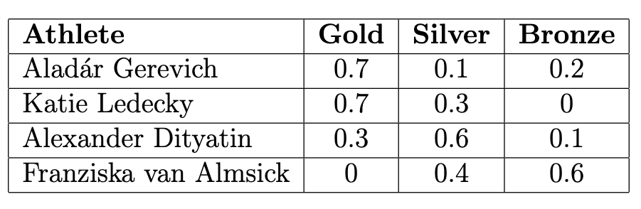
Which type of data visualization is most appropriate to compare two athlete’s medal distributions?
overlaid histogram
overlaid bar chart
overlaid line plot
Answer: overlaid bar chart
Here, we are plotting the data of 2 athletes, comparing the medal distributions. Gold, silver, and bronze medals are categorical variables, while the proportion of these won is a quantitative value. A bar chart is the only kind of plot that involves categorical data with quantitative data. Since there are 2 athletes, the most appropriate plot is an overlaid bar chart. The overlapping bars would help compare the difference in their distributions.
The average score on this problem was 73%.
Among the other athletes in the table above, whose medal distribution has the largest total variation distance (TVD) to Aladár Gerevich’s distribution?
Katie Ledecky
Alexander Dityatin
Franziska van Almsick
Answer: Franziska van Almsick
The Total Variation Distance (TVD) of two categorical distributions is the sum of the absolute differences of their proportions, all divided by 2. We can apply the TVD formula to these distributions: The TVD between Katie Ledecky and Aladar Gerevich is given by \frac{1}{2} \cdot (|0.7 - 0.7| + |0.1 - 0.3| + |0.2 - 0|) = \frac{0.4}{2} = 0.2. The TVD between Alexander Dityatin and Aladar Gerevich is given by \frac{1}{2} \cdot (|0.7 - 0.3| + |0.1 - 0.6| + |0.2 - 0.1|) = \frac{1}{2} = 0.5. And finally, the TVD between Franziska van Almsick and Aladar Gerevich is given by \frac{1}{2} \cdot (|0.7 - 0| + |0.1 - 0.4| + |0.2 - 0.6|) = \frac{1.4}{2} = 0.7. So, Franziska van Almsick has the largest TVD to Gerevich’s distribution.
The average score on this problem was 92%.
Suppose Pallavi earns 10 Olympic medals in such a way that the TVD between Pallavi’s medal distribution and Aladár Gerevich’s medal distribution is as large as possible. What is Pallavi’s medal distribution?
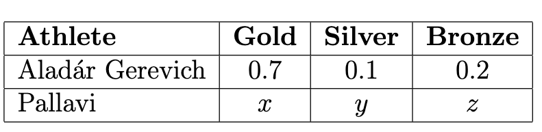
Answer: x=0, y=1, z=0
Intuitively, can maximize the TVD between the distributions by putting all of Pallavi’s medals in the category which Gerevich won the least of, so x = 0, y = 1, z = 0. Moving any of these medals to another category would decrease the TVD, since that would mean that all of Pallavi’s medal proportions would get closer to Gerevich’s (Silver is decreasing, getting closer, and Gold and Bronze are increasing, which makes them closer as well).
The average score on this problem was 72%.
More generally, suppose medal_dist is an array of length
three representing an athlete’s medal distribution. Which of the
following expressions gives the maximum possible TVD between
medal_dist and any other distribution?
medal_dist.max()
medal_dist.min()
1 - medal_dist.max()
1 - medal_dist.min()
np.abs(1 - medal_dist).sum()/2
Answer: 1 - medal_dist.min()
Similar to part c, we know that the TVD is maximized by placing all
the medals of competitor A into the category in which competitor B has
the lowest proportion of medals. If we place all of competitor A’s
medals into this bin, the difference between the two distributions for
this variable will be 1 - medal_dist.min() In the other
bins, competitor A has no medals (making all their values 0), and
competitor B has the remainder of their medals, which is
1 - medal_dist.min(). So, in total, the TVD is given by
\frac{1}{2} \cdot 2 \cdot
1 - medal_dist.min() =
1 - medal_dist.min().
The average score on this problem was 56%.
Bill claims that San Diego is sunny 60% of the year, but you think the percentage is higher. You decide to test the validity of Bill’s claim by running a hypothesis test.
Both your null and alternative hypotheses will take this form:
The percentage of sunny days in San Diego is ______ 60%.
(i) For the null hypothesis, how should we fill in the blank?
equal to
not equal to
greater than
less than
(ii) For the alternative hypothesis, how should we fill in the blank?
equal to
not equal to
greater than
less than
Answer (i): equal to
The average score on this problem was 89%.
Answer (ii): greater than
The average score on this problem was 75%.
Say that in 2023, San Diego had 235 sunny days. Using the number of
sunny days per year as the test statistic, fill in the following code to
run the hypothesis test and store the p-value of your test in
p_val. We’ll assume that all years have 365 days.
    observed_stat = ___(w)___
    results = np.array([])

    for i in np.arange(10000):
        result = np.___(x)___(365, ___(y)___)[0]
        results = np.append(results, result)

p_val = np.count_nonzero(results __(z)__ observed_stat) / 10000Answer (w): 235
The average score on this problem was 58%.
Answer (x): random.multinomial
The average score on this problem was 93%.
Answer (y): [0.6, 0.4]
The average score on this problem was 65%.
Answer (z): >=
The average score on this problem was 67%.
Suppose the p-value of this hypothesis test is 0.1. Which of the following statements is a correct interpretation of this p-value?
If the null hypothesis is true, there is a 10% chance of obtaining a test statistic equal to the observed statistic.
If the null hypothesis is true, there is a 90% chance of obtaining a test statistic equal to the observed statistic.
If the null hypothesis is true, there is a 10% chance of obtaining a test statistic equal to, or at least as extreme as, the observed statistic.
If the alternative hypothesis is true, there is a 90% chance of obtaining a test statistic equal to, or at least as extreme as, the observed statistic.
Answer: If the null hypothesis is true, there is a 10% chance of obtaining a test statistic equal to, or at least as extreme as, the observed statistic.
The average score on this problem was 76%.
Professor Minerva McGonagall, head of Gryffindor, may also be awarding house points unfairly. For this question, we’ll assume that all four of the houses contain the same number of students, and we’ll investigate whether McGonagall awards points equally to all four houses.
Below is the distribution of points that Professor McGonagall awarded during the last academic year.
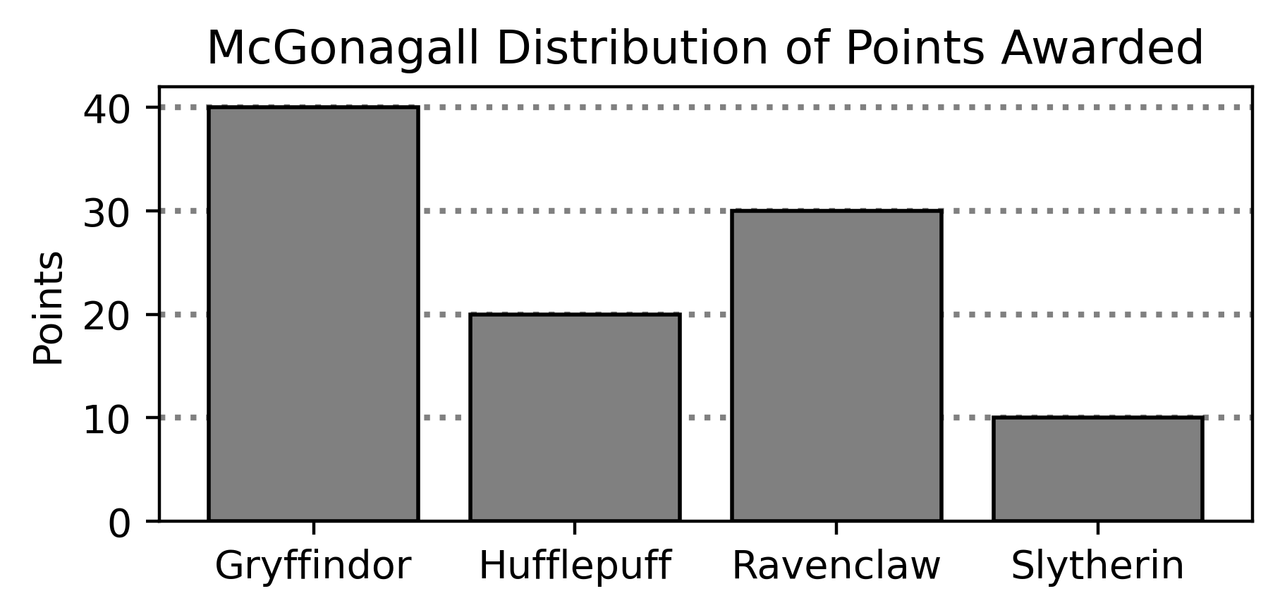
You want to test the following hypotheses:
Null Hypothesis: The distribution of points awarded by Professor McGonagall is uniform across all of the houses.
Alternative Hypothesis: The distribution of points awarded by Professor McGonagall is not uniform across all of the houses.
Which of the following test statistics is appropriate for this hypothesis test? Select all that apply.
The absolute difference between the number of points awarded to Gryffindor and the proposed proportion of points awarded to Gryffindor.
The difference between the number of points awarded to the house with the most points and the house with the least points.
The sum of the squared differences in proportions between
McGonagall’s distribution and [0.5, 0.5, 0.5, 0.5].
The sum of the differences in proportions between McGonagall’s
distribution and [0.25, 0.25, 0.25, 0.25].
The sum of the squared differences in proportions between
McGonagall’s distribution and [0.25, 0.25, 0.25, 0.25].
None of the above.
Answer: Option 2 and 5.
This problem is trying to find test statistics that can be used to distinguish when the data is better supported by the alternative. Since the alternative hypothesis simply states “is not uniform across all of the houses”, it is not crucial to look for individual differences between houses but rather the general relationship of points awarded to all houses.
Option 1: This option only tells us information about Gryffindor but doesn’t tell us anything about inequalities between other houses. For example,e if Gryffindor received 25% of the points and Slytherin received the other 75% of the points we would not be able to tell this apart from the case when all houses received 25% of the points.
Option 2: When the points are distributed normally we would expect that all the houses receive about the same amount and therefore the difference of points would be near 0. However, if one house is gaining more points than the rest of the houses then the number of points between the top and lowest house we be greater than 0. Therefore we are “measuring” the alternative.
Option 3: This test statistic measures the sum of
the squared differences in proportions between McGonagall’s distribution
and [0.5, 0.5, 0.5, 0.5]. However,
[0.5, 0.5, 0.5, 0.5] does not represent a valid probability
distribution because the total sum exceeds 1. As a result, this test
statistic is not meaningful in assessing whether the point distribution
is uniform across houses.
Option 4: When we measure the sum of the
differences, the information on “how close” the data is to the
alternative can be unseen. For example, a distribution of
[0.25, 0.25, 0.25, 0.25] is what we’d expect under the null
and a distribution of [0.0, 0.5, 0.0, 0.5] would support
the alternative. However, using this test statistic we would see a
result of 0 therefore not differentiating them.
Option 5: Under the null hypothesis
[0.25, 0.25, 0.25, 0.25] is the “expected” distribution.
Additionally, since the alternative hypothesis states that McGongall’s
assignments are not uniform (aka is the distribution of points
non-uniform), a house supports the alternative if its points are
significantly less than or greater than 0.25.
Squaring the differences allows the test statistic to be greater in
either case and therefore would be a valid statistic.
The average score on this problem was 78%.
For the rest of this problem, we will use the following test statistic:
The sum of the absolute differences in proportions between
McGonagall’s distribution and
[0.25, 0.25, 0.25, 0.25].
Choose the correct way to implement the function
calculate_test_stat, which takes in two distributions as
arrays and returns the value of this test statistic.
    def calculate_test_stat(dist_1, dist_2):
        return _____
np.abs(sum(dist_1 - dist_2)).
abs(sum(dist_1 - dist_2)).
sum(np.abs(dist_1 - dist_2)).
sum(abs(dist_1 - dist_2)).
Answer:
sum(np.abs(dist_1 - dist_2))
A valid test statistic in this problem would find how far
dist_1 differs from dist_2. Since we’re
looking at “how
different”) the distributions are, we need to take the absolute
value (aka a measure of distance/difference) and then add them up.
np.abs() needs to be used over abs() because
dist_1 and dist_2 are arrays
and the built-in function abs only works for individual
numbers.
The average score on this problem was 84%.
(10 pts) Fill in the blanks in the code below so that
simulated_ts is an array containing 10,000 simulated values
of the test statistic under the null. Note that your answer to blank
(c) is used in more than one place in the
code.
    mc_gon = np.arange(__(a)__) # Careful: np.arange, not np.array!
    null = np.array([0.25, 0.25, 0.25, 0.25])
    observed_ts = calculate_test_stat(__(b)__)

    simulated_ts = np.array([])

    for i in np.arange(10000):
        sim = np.random.multinomial(__(c)__, __(d)__) / __(c)__
        one_simulated_ts = calculate_test_stat(__(e)__)
        simulated_ts = np.append(simulated_ts, one_simulated_ts)
What goes in blank (a)?
Answer: 0.1, 0.5, 0.1 (or equivalent)
Based on the distribution shown in the bar chart above, we want our
resulting array to contain the proportions
[0.4, 0.2, 0.3, 0.1] (40/100 for Gryffindor, 20/100 for
Hufflepuff, 30/100 for Ravenclaw, and 10/100 for Slytherin). Note that
the order of these proportions does not matter because: 1) we are
calculating the absolute difference between each value and the null
proportion (0.25), and 2) we will sum all the differences together.
Since these proportions are incrementally increasing, we can use
np.arange() to construct mc_gon. There are
multiple correct approaches to this problem, as long as the resulting
array contains all four proportions. Some alternative correct approaches
include: - np.arange(0.4, 0.0, -0.1) -
np.arange(0.1, 0.41, 0.1) (The middle argument can be any
value greater than 0.4 and less than or equal to 0.5)
The average score on this problem was 57%.
What goes in blank (b)?
Answer: null, mc_gon
Note that the order of mc_gon and null does
not matter, as calculate_test_stat calculates the absolute
difference between the two.
The average score on this problem was 78%.
What goes in blank (c)?
Answer: 100
Blank (c) represents the total number of trials in each simulated sample. Using 100 ensures that each sample is large enough to approximate the expected proportions while maintaining computational efficiency. Additionally, (c) is used to divide all values, converting counts into proportions.
The average score on this problem was 48%.
What goes in blank (d)?
Answer: null
Blank (d) is null because each simulated sample is generated under
the null hypothesis. This means the probabilities used in
np.random.multinomial should match the expected proportions
from the null distribution.
The average score on this problem was 77%.
What goes in blank (e)?
Answer: sim, null
Note that the order of null and sim does
not matter, as calculate_test_stat calculates the absolute
difference between the two.
The average score on this problem was 67%.
Fill in the blank so that reject_null evaluates to
True if we reject the null hypothesis at the 0.05 significance level, and
False otherwise.
reject_null = __(f)__Answer:
(simulated_ts >= observed_ts).mean() <= 0.05
reject_null should evaluate to a boolean statement
therefore we must test whether our p-value)
is less than or equal to 0.05. Taking the mean of
(simulated_ts >= observed_ts) tells us the proportion of
simulated test statistics that are equal to the value that was observed
in the data or is even further in the direction of the alternative.
The average score on this problem was 64%.
Your friend performs the same hypothesis test as you, but uses the total variation distance (TVD) as their test statistic instead of the one described in the problem. Which of the following statements is true?
Your friend’s simulated statistics will be larger than yours, because TVD accounts for the magnitude and direction of the differences in proportions.
Your friend’s simulated statistics will be larger than yours, but not because it accounts for the magnitude and direction of the differences in proportions.
Your friend’s simulated statistics will be smaller than yours, because TVD accounts for the magnitude and direction of the differences in proportions.
Your friend’s simulated statistics will be smaller than yours, but not because it accounts for the magnitude and direction of the differences in proportions.
There is no relationship between the statistic you used and the statistic your friend used (TVD).
Answer: Option 4.
TVD) is calculated by taking the sum of the absolute differences of two proportions, all divided by 2. Therefore the only difference between TVD and our test statistic is the fact that TVD is divided by 2 (which would make it smaller). Meaning that the reason it is smaller is not related to magnitude or direction.
The average score on this problem was 63%.
Using his years of statistical skill and investigative prowess, Detective Peter decides to conduct a permutation test to determine whether one of the two graders was significantly harsher than the other. He has Jeffrey’s scores and Kate’s scores and no assumed knowledge of the population distribution of scores. Which of the following best explains both why a permutation test is appropriate here and how it should be done?
We have two samples and want to test whether they came from the same distribution. Under the null hypothesis, we simulate by shuffling the group labels, since if the distributions are the same the labels shouldn’t matter.
We have two samples and want to test whether they came from the same distribution. Under the null hypothesis, we simulate by resampling with replacement from the combined 50 scores to form two new groups.
We want to compare Jeffrey’s scores against a known population distribution of Quiz 3 scores. Under the null hypothesis, we simulate by shuffling scores and recomputing the test statistic.
Shuffling the grader labels generates two new random samples from the population of all possible Quiz 3 scores, letting us estimate the sampling distribution of the test statistic.
Answer: We have two samples and want to test whether they came from the same distribution. Under the null hypothesis, we simulate by shuffling the group labels, since if the distributions are the same the labels shouldn’t matter.
A permutation test is appropriate when we want to compare two samples
and the null hypothesis is that they come from the same distribution
(labels are arbitrary). We simulate under the null by randomly permuting
which scores are assigned to which grader — i.e., shuffling the
grader labels — and recomputing the test statistic each
time. Resampling with replacement from the pooled data would be
bootstrap-style, not the usual permutation scheme for this setup.
The average score on this problem was 83%.
Detective Peter moves forward with his permutation test to compare Jeffrey’s and Kate’s scores. He suspects that Jeffrey is the harsher grader — that is, Jeffrey’s scores tend to be lower than Kate’s, and wants to determine if there is evidence to support this.
Which null and alternative hypothesis pair is most appropriate?
Null: Jeffrey and Kate gave scores from the same distribution. Alt: Jeffrey gave scores from a distribution with a smaller mean than Kate’s.
Null: Jeffrey’s scores come from a known population with mean 70. Alt: Jeffrey’s scores do not come from a population with mean 70.
Null: Jeffrey and Kate gave scores from the same distribution. Alt: The distribution of Jeffrey’s scores is entirely lower than the distribution of Kate’s scores.
Null: The mean score from Jeffrey equals the mean score from Kate. Alt: The mean score from Jeffrey does not equal the mean score from Kate.
Answer: Null: Jeffrey and Kate gave scores from the same distribution. Alt: Jeffrey gave scores from a distribution with a smaller mean than Kate’s.
We want a one-sided alternative that Jeffrey is harsher (lower mean). The permutation test framework compares whether the two samples could have come from the same distribution (null); the alternative should encode “Jeffrey’s distribution has a smaller mean than Kate’s,” not a two-sided difference in means only, and not that every Jeffrey score is below every Kate score.
The average score on this problem was 66%.
For testing whether Jeffrey is the harsher grader, which of the following could be used as a test statistic to get a p-value directly from its empirical distribution under the null hypothesis? Select all that are correct.
The difference in group means: Kate’s mean minus Jeffrey’s mean.
The difference in group means: Jeffrey’s mean minus Kate’s mean.
The absolute difference between the two groups’ mean scores.
The total variation distance between the two graders’ score distributions.
None of the above.
Answer: The difference in group means: Kate’s mean minus Jeffrey’s mean; The difference in group means: Jeffrey’s mean minus Kate’s mean.
Either signed difference in means is a valid test statistic: under the null (same distribution), permuting labels gives an empirical null distribution for that statistic, and the p-value is computed from how extreme the observed value is. One-sided conclusions depend on which sign you use and how you define “as extreme.” The absolute difference corresponds to a two-sided comparison of means. TVD could compare distributions but is not required here; the problem asks which could be used — the two mean differences are standard choices.
The average score on this problem was 75%.
Overall, Detective Peter determined that Jeffrey’s offenses are grave enough: Peter travels all the way back to Tutorlandia to consult the great council of tutors on what Jeffrey’s penance should be. It was decided that Jeffrey must explain to the class what the total variation distance (TVD) measures. Which of the following is a correct description of the TVD?
The difference between two group means.
A measure of how different two distributions (of any type) are.
A measure of how different two numeric distributions are.
A measure of how different two categorical distributions are.
The proportion of simulated statistics that are at least as extreme as the observed value.
The width of a 95% confidence interval.
Answer: A measure of how different two categorical distributions are.
TVD compares two distributions on a finite set of categories by summing half the absolute differences of the proportions in each category. It is defined for categorical data, not as a general measure for arbitrary numeric distributions.
The average score on this problem was 66%.