← return to practice.dsc10.com
Below are practice problems tagged for Lecture 21 (rendered directly from the original exam/quiz sources).
At the San Diego Model Railroad Museum, there are different admission prices for children, adults, and seniors. Over a period of time, as tickets are sold, employees keep track of how many of each type of ticket are sold. These ticket counts (in the order child, adult, senior) are stored as follows.
admissions_data = np.array([550, 1550, 400])Complete the code below so that it creates an array
admissions_proportions with the proportions of tickets sold
to each group (in the order child, adult, senior).
def as_proportion(data):
    return __(a)__

admissions_proportions = as_proportion(admissions_data)
What goes in blank (a)?
Answer: data/data.sum()
To calculate proportion for each group, we divide each value in the array (tickets sold to each group) by the sum of all values (total tickets sold). Remember values in an array can be processed as a whole.
The average score on this problem was 95%.
The museum employees have a model in mind for the proportions in which they sell tickets to children, adults, and seniors. This model is stored as follows.
model = np.array([0.25, 0.6, 0.15])We want to conduct a hypothesis test to determine whether the admissions data we have is consistent with this model. Which of the following is the null hypothesis for this test?
Child, adult, and senior tickets might plausibly be purchased in proportions 0.25, 0.6, and 0.15.
Child, adult, and senior tickets are purchased in proportions 0.25, 0.6, and 0.15.
Child, adult, and senior tickets might plausibly be purchased in proportions other than 0.25, 0.6, and 0.15.
Child, adult, and senior tickets, are purchased in proportions other than 0.25, 0.6, and 0.15.
Answer: Child, adult, and senior tickets are purchased in proportions 0.25, 0.6, and 0.15. (Option 2)
Recall, null hypothesis is the hypothesis that there is no significant difference between specified populations, any observed difference being due to sampling or experimental error. So, we assume the distribution is the same as the model.
The average score on this problem was 88%.
Which of the following test statistics could we use to test our hypotheses? Select all that could work.
sum of differences in proportions
sum of squared differences in proportions
mean of differences in proportions
mean of squared differences in proportions
none of the above
Answer: sum of squared differences in proportions, mean of squared differences in proportions (Option 2, 4)
We need to use squared difference to avoid the case that large positive and negative difference cancel out in the process of calculating sum or mean, resulting in small sum of difference or mean of difference that does not reflect the actual deviation. So, we eliminate Option 1 and 3.
The average score on this problem was 77%.
Below, we’ll perform the hypothesis test with a different test statistic, the mean of the absolute differences in proportions.
Recall that the ticket counts we observed for children, adults, and
seniors are stored in the array
admissions_data = np.array([550, 1550, 400]), and that our
model is model = np.array([0.25, 0.6, 0.15]).
For our hypothesis test to determine whether the admissions data is
consistent with our model, what is the observed value of the test
statistic? Give your answer as a number between 0 and 1, rounded to
three decimal places. (Suppose that the value you calculated is assigned
to the variable observed_stat, which you will use in later
questions.)
Answer: 0.02
We first calculate the proportion for each value in
admissions_data \frac{550}{550+1550+400} = 0.22 \frac{1550}{550+1550+400} = 0.62 \frac{400}{550+1550+400} = 0.16 So, we have
the distribution of the admissions_data
Then, we calculate the observed value of the test statistic (the mean of the absolute differences in proportions) \frac{|0.22-0.25|+|0.62-0.6|+|0.16-0.15|}{number\ of\ goups} =\frac{0.03+0.02+0.01}{3} = 0.02
The average score on this problem was 82%.
Now, we want to simulate the test statistic 10,000 times under the
assumptions of the null hypothesis. Fill in the blanks below to complete
this simulation and calculate the p-value for our hypothesis test.
Assume that the variables admissions_data,
admissions_proportions, model, and
observed_stat are already defined as specified earlier in
the question.
simulated_stats = np.array([])
for i in np.arange(10000):
    simulated_proportions = as_proportions(np.random.multinomial(__(a)__, __(b)__))
    simulated_stat = __(c)__
    simulated_stats = np.append(simulated_stats, simulated_stat)

p_value = __(d)__
What goes in blank (a)? What goes in blank (b)? What goes in blank (c)? What goes in blank (d)?
Answer: (a) admissions_data.sum() (b)
model (c)
np.abs(simulated_proportions - model).mean() (d)
np.count_nonzero(simulated_stats >= observed_stat) / 10000
Recall, in np.random.multinomial(n, [p_1, ..., p_k]),
n is the number of experiments, and
[p_1, ..., p_k] is a sequence of probability. The method
returns an array of length k in which each element contains the number
of occurrences of an event, where the probability of the ith event is
p_i.
We want our simulated_proportion to have the same data
size as admissions_data, so we use
admissions_data.sum() in (a).
Since our null hypothesis is based on model, we simulate
based on distribution in model, so we have
model in (b).
In (c), we compute the mean of the absolute differences in
proportions. np.abs(simulated_proportions - model) gives us
a series of absolute differences, and .mean() computes the
mean of the absolute differences.
In (d), we calculate the p_value. Recall, the
p_value is the chance, under the null hypothesis, that the
test statistic is equal to the value that was observed in the data or is
even further in the direction of the alternative.
np.count_nonzero(simulated_stats >= observed_stat) gives
us the number of simulated_stats greater than or equal to
the observed_stat in the 10000 times simulations, so we
need to divide it by 10000 to compute the proportion of
simulated_stats greater than or equal to the
observed_stat, and this gives us the
p_value.
The average score on this problem was 79%.
True or False: the p-value represents the probability that the null hypothesis is true.
True
False
Answer: False
Recall, the p-value is the chance, under the null hypothesis, that the test statistic is equal to the value that was observed in the data or is even further in the direction of the alternative. It only gives us the strength of evidence in favor of the null hypothesis, which is different from “the probability that the null hypothesis is true”.
The average score on this problem was 64%.
The new statistic that we used for this hypothesis test, the mean of
the absolute differences in proportions, is in fact closely related to
the total variation distance. Given two arrays of length three,
array_1 and array_2, suppose we compute the
mean of the absolute differences in proportions between
array_1 and array_2 and store the result as
madp. What value would we have to multiply
madp by to obtain the total variation distance
array_1 and array_2? Give your answer as a
number rounded to three decimal places.
Answer: 1.5
Recall, the total variation distance (TVD) is the sum of the absolute differences in proportions, divided by 2. When we compute the mean of the absolute differences in proportions, we are computing the sum of the absolute differences in proportions, divided by the number of groups (which is 3). Thus, to get TVD, we first multiply our current statistics (the mean of the absolute differences in proportions) by 3, we get the sum of the absolute differences in proportions. Then according to the definition of TVD, we divide this value by 2. Thus, we have \text{current statistics}\cdot 3 / 2 = \text{current statistics}\cdot 1.5.
The average score on this problem was 65%.
The table below shows how many movies in each of four genres Jack and Eric have seen. What is the total variation distance (TVD) between Jack and Eric’s distribution of movies by genre?
"Musical" |
"Comedy" |
"Action" |
"Horror" |
Total | |
|---|---|---|---|---|---|
| Jack | 2 | 14 | 2 | 2 | 20 |
| Eric | 55 | 15 | 15 | 15 | 100 |
Answer: 0.55
The average score on this problem was 25%.
Oren’s favorite bakery in San Diego is Wayfarer. After visiting frequently, he decides to learn how to make croissants and baguettes himself, and to do so, he books a trip to France.
Oren is interested in estimating the mean number of sunshine hours in
July across all 10,000+ cities in France. Using the 16 French cities in
sun, Oren constructs a 95% Central Limit Theorem
(CLT)-based confidence interval for the mean sunshine hours of all
cities in France. The interval is of the form [L, R], where L and R are
positive numbers.
Which of the following expressions is equal to the standard deviation
of the number of sunshine hours of the 16 French cities in
sun?
R - L
\frac{R - L}{2}
\frac{R - L}{4}
R + L
\frac{R + L}{2}
\frac{R + L}{4}
Answer: R - L
Note that the 95% CI is of the form of the following:
[\text{Sample Mean} - 2 \cdot \text{SD of Distribution of Possible Sample Means}, \text{Sample Mean} + 2 \cdot \text{SD of Distribution of Possible Sample Means}]
This making its width 4 \cdot \text{SD of Distribution of Possible Sample Means}. We can use the square root law, the fact that we can use our sample’s SD as an estimate of our population’s SD when creating a confidence interval, and the fact that the sample size is 16, to re-write the width as:
\begin{align*} \text{width} &= 4 \cdot \text{SD of Distribution of Possible Sample Means} \\ &= 4 \cdot \left(\frac{\text{Population SD}}{\sqrt{\text{Sample Size}}}\right) \\ &\approx 4 \cdot \left(\frac{\text{Sample SD}}{\sqrt{\text{Sample Size}}}\right) \\ &= 4 \cdot \left(\frac{\text{Sample SD}}{4}\right) \\ &= \text{Sample SD} \end{align*}
Since \text{width} = \text{Sample SD}, and since \text{width} = R - L, we have that \text{Sample SD} = R - L.
The average score on this problem was 27%.
True or False: There is a 95% chance that the interval [L, R] contains the mean number of sunshine
hours in July of all 16 French cities in sun.
True
False
Answer: False
[L, R] contains the sample mean for sure, since it is centered at the sample mean. There is no probability associated with this fact since neither [L, R] nor the sample mean are random (given that our sample has already been drawn).
The average score on this problem was 62%.
True or False: If we collected 1,000 new samples of 16 French cities and computed the mean of each sample, then about 95% of the new sample means would be contained in [L, R].
True
False
Answer: False
It is true that if we collected many samples and used each one to make a 95% confidence interval, about 95% of those confidence intervals would contain the population mean. However, that’s not what this statement is addressing. Instead, it’s asking whether the one interval we created in particular, [L,R], would contain 95% of other samples’ means. In general, there’s no guarantee of the proportion of means of other samples that would fall in [L, R]; for instance, it’s possible that the sample that we used to create [L, R] was not a representative sample.
The average score on this problem was 42%.
True or False: If we collected 1,000 new samples of 16 French cities and created a 95% confidence interval using each one, then chose one of the 1,000 new intervals at random, the chance that the randomly chosen interval contains the mean sunshine hours in July across all cities in France is approximately 95%.
True
False
Answer: True
It is true that if we collected many samples and used each one to make a 95% confidence interval, about 95% of those confidence intervals would contain the population mean, as we mentioned above. So, if we picked one of those confidence intervals at random, there’s an approximately 95% chance it would contain the population mean.
The average score on this problem was 57%.
True or False: The interval [L, R] is centered at the mean number of sunshine hours in July across all cities in France.
True
False
Answer: False
It is centered at our sample mean, which is the mean sunshine hours
in July across all cities in France in sun, but not
necessarily at the population mean. We don’t know where the population
mean is!
The average score on this problem was 58%.
In addition to creating a 95% CLT-based confidence interval for the mean sunshine hours of all cities in France, Oren would like to create a 72% bootstrap-based confidence interval for the mean sunshine hours of all cities in France.
Oren resamples from the 16 French sunshine hours in sun
10,000 times and creates an array named french_sunshine
containing 10,000 resampled means. He wants to find the left and right
endpoints of his 72% confidence interval:
    boot_left = np.percentile(french_sunshine, __(a)__)
boot_right = np.percentile(french_sunshine, __(b)__)Fill in the blanks so that boot_left and
boot_right evaluate to the left and right endpoints of a
72% confidence interval for the mean sunshine hours in July across all
cities in France.
What goes in blanks (a) and (b)?
Answer: (a): 14, (b): 86
A 72% confidence interval is constructed by taking the middle 72% of the distribution of resampled means. This means we need to exclude 100\% - 72\% = 28\% of values – the smallest 14% and the largest 14%. Blank (a), then, is 14, and blank (b) is 100 - 14 = 86.
The average score on this problem was 81%.
Suppose we are interested in testing the following pair of hypotheses.
Null Hypothesis: The mean number of sunshine hours of all cities in France in July is equal to 225.
Alternative Hypothesis: The mean number of sunshine hours of all cities in France in July is not equal to 225.
Suppose that when Oren uses [boot_left, boot_right], his
72% bootstrap-based confidence interval, he fails to reject the null
hypothesis above. If that’s the case, then when using [L, R], his 95% CLT-based confidence
interval, what is the conclusion of his hypothesis test?
Reject the null
Fail to reject the null
Impossible to tell
Answer: Impossible to tell
First, remember that we fail to reject the null whenever the parameter stated in the null hypothesis (225 in this case) is in the interval. So we’re told 225 is in the 72% bootstrapped interval. There’s a possibility that the 72% bootstrapped confidence interval isn’t completely contained within the 95% CLT interval, since the specific interval we get back with bootstrapping depends on the random resamples we get. What that means is that it’s possible for 225 to be in the 72% bootstrapped interval but not the 95% CLT interval, and it’s also possible for it to be in the 95% CLT interval. Therefore, given no other information it’s impossible to tell.
The average score on this problem was 47%.
Suppose that Oren also creates a 72% CLT-based confidence interval
for the mean sunshine hours of all cities in France in July using the
same 16 French cities in sun he started with. When using
his 72% CLT-based confidence interval, he fails to reject the null
hypothesis above. If that’s the case, then when using [L, R], what is the conclusion of his
hypothesis test?
Reject the null
Fail to reject the null
Impossible to tell
Answer: Fail to reject the null
If 225 is in the 72% CLT interval, it must be in the 95% CLT interval, since the two intervals are centered at the same location and the 95% interval is just wider than the 72% interval. The main difference between this part and the previous one is the fact that this 72% interval was made with the CLT, not via bootstrapping, even though they’re likely to be similar.
The average score on this problem was 72%.
True or False: The significance levels of both hypothesis tests described in part (h) are equal.
True
False
Answer: False
When using a 72% confidence interval, the significance level, i.e. p-value cutoff, is 28%. When using a 95% confidence interval, the significance level is 5%.
The average score on this problem was 62%.
We want to use the data in apts to test the following
hypotheses:
While we could answer this question with a permutation test, in this problem we will explore another way to test these hypotheses. Since this is a question of whether two samples come from the same unknown population distribution, we need to construct a “population” to sample from. We will construct our “population” in the same way as we would for a permutation test, except we will draw our sample differently. Instead of shuffling, we will draw our two samples with replacement from the constructed “population”. We will use as our test statistic the difference in means between the two samples (in the order UTC minus elsewhere).
Suppose the data in apts, which has 800 rows, includes
85 apartments in UTC. Fill in the blanks below so that
p_val evaluates to the p-value for this hypothesis test,
which we will test according to the strategy outlined above.
diffs = np.array([])
for i in np.arange(10000):
    utc_sample_mean = __(a)__
    elsewhere_sample_mean = __(b)__
    diffs = np.append(diffs, utc_sample_mean - elsewhere_sample_mean)
observed_utc_mean = __(c)__
observed_elsewhere_mean = __(d)__
observed_diff = observed_utc_mean - observed_elsewhere_mean
p_val = np.count_nonzero(diffs __(e)__ observed_diff) / 10000Answer:
apts.sample(85, replace=True).get("Rent").mean()apts.sample(715, replace=True).get("Rent").mean()apts[apts.get("neighborhood")=="UTC"].get("Rent").mean()apts[apts.get("neighborhood")!="UTC"].get("Rent").mean()>=For blanks (a) and (b), we can gather from context (hypothesis test
description, variable names, and being inside of a for loop) that this
portion of our code needs to repeatedly generate samples of size 85 (the
number of observations in our dataset that are from UTC) and size 715
(the number of observations in our dataset that are not from UTC). We
will then take the means of these samples and assign them to
utc_sample_mean and elsewhere_sample_mean. We
can generate these samples, with replacement, from the rows in our
dataframe, hinting that the correct code for blanks (a) and (b) are:
apts.sample(85, replace=True).get("Rent").mean() and
apts.sample(715, replace=True).get("Rent").mean().
For blanks (c) and (d), this portion of the code needs to take our
original dataframe and gather the observed means for apartments from UTC
and apartments not from UTC. We can achieve this by querying our
dataframe, grabbing the rent column, and taking the mean. This implies
our correct code for blanks (c) and (d) are:
apts[apts.get("neighborhood")=="UTC"].get("Rent").mean()
and
apts[apts.get("neighborhood")!="UTC"].get("Rent").mean().
For blank (e), we need to determine, based off of our null and
alternative hypotheses, how we should compare the differences in found
in our simulations against our observed difference. The alternative
indicates that that values of rent of apartments in UTC are
higher than the rent of other apartments in other
neighborhoods. Since the observed statistic is calculated by
observed_utc_mean - observed_elsewhere_mean, we want to use
>= in (e) since greater values of diff
indicate that observed_utc_mean is greater than
observed_elsewhere_mean which is in the direction of the
alternative hypothesis.
The average score on this problem was 70%.
Now suppose we tested the same hypothesses with a permutation test using the same test statistic. Which of your answers above (part a) would need to change? Select all that apply.
blank (a)
blank (b)
blank (c)
blank (d)
blank (e)
None of these.
Answer: Blanks (a) and (b) would need to change. For
a permutation test, we would shuffle the labels in our apts
dataset and find the utc_sample_mean and
elsewhere_sample_mean of this new shuffled dataset. Note
that this process is done without replacement and that
both of these sample means are calculated from the same shuffle
of our dataset.
As it currently stands, our code for blanks (a) and (b) do not reflect this; the current process is sampling with replacement from two different shuffles of our dataset. So, blanks (a) and (b) must change.
The average score on this problem was 93%.
Now suppose we test the following pair of hypotheses.
Then we can test this pair of hypotheses by constructing a 95% confidence interval for a parameter and checking if some particular number, x, falls in that confidence interval. To do this:
What parameter should we construct a 95% confidence interval for? Your answer should be a phrase or short sentence.
What is the value of x? Your answer should be a number.
Suppose x is in the 95% confidence interval we create. Select all valid conclusions below.
We reject the null hypothesis at the 5% significance level.
We reject the null hypothesis at the 1% significance level.
We fail to reject the null hypothesis at the 5% significance level.
We fail to reject the null hypothesis at the 1% significance level.
Answer:
For (i), we need to construct a confidence interval for a parameter that allows us to make assessments about our null and alternative hypotheses. Since these two hypotheses discuss whether or not there exists a difference, on average, for rents of apartments in UTC versus rents of apartments elsewhere, our parameter should be: the difference in rent for apartments in UTC and apartments elsewhere on average, or vice versa (The average rent of an apartment in UTC minus the average rent of an apartment elsewhere, or vice versa.)
For (ii), x must be 0 because the value zero holds special significance in our confidence interval; the inclusion of zero within our confidence interval suggests that “there is no difference between rent of apartments in UTC and apartments elsewhere, on average”. Whether or not zero is included within our confidence interval tells us whether we should fail to reject or reject the null hypothesis.
For (iii), if x = 0 lies within our 95% confidence interval, it suggests that there is a sizable chance that there is no difference between rent of apartments in UTC and apartments elsewhere, on average, which is a conclusion in favor of our null hypothesis; this means that any options which reject the null hypothesis, such as the 1st and 2st options, are wrong. The 3rd option (correctly) fails to the reject the null hypothesis at the 5% significance level, which is exactly what a 95% confidence interval that includes x = 0 would support. The 4th option is also correct because any evidence weak enough to fail to reject the null hypothesis at the 5% significance level will also fail at a tighter, more rigorous significance level (such as 1%).
The average score on this problem was 36%.
The average score on this problem was 53%.
The average score on this problem was 77%.
You want to determine if the bikes for sale locally have the
following distribution of "style": "electric"
(15%), "mountain" (20%), "road" (40%),
"hybrid" (20%), and "recumbent" (5%). You want
to use the 500 rows of bikes to test the following
hypotheses:
Null: Bikes for sale locally are randomly drawn from the proposed distribution.
Alt: Bikes for sale locally are not randomly drawn from the proposed distribution.
Suppose that in bikes, the "style" column
is distributed as follows: "electric" (20%),
"mountain" (20%), "road" (30%),
"hybrid" (20%), and "recumbent" (10%).
Let’s do a hypothesis test with total variation distance (TVD) as the test statistic. Fill in the blanks below to complete a simulation that calculates 10,000 TVDs under the null hypothesis.
def total_variation_distance(distr1, distr2):
    return __(a)__

proposed = np.array([0.15, 0.20, 0.40, 0.20, 0.05])
observed = np.array([0.20, 0.20, 0.30, 0.20, 0.10])
tvds = np.array([])
for i in np.arange(10000):
    simulated = np.random.multinomial(__(b)__, __(c)__) / 500
    new_tvd = total_variation_distance(__(d)__, __(e)__)
tvds = np.append(tvds, new_tvd)Answer:
(a): np.abs((distr1 - distr2)).sum() / 2
(b): 500
(c): proposed
(d): simulated
(e): proposed
The average score on this problem was 78%.
Fill in the blanks below so that observed_tvd
corresponds to the observed value of the test statistic for this
hypothesis test.
observed_tvd = total_variation_distance(__(f)__, __(g)__)Answer:
(f): observed
(g): proposed
The average score on this problem was 83%.
Which of the following correctly calculates the p-value for this hypothesis test?
p_value = np.count_nonzero(tvds >= observed_tvd) / len(observed)
p_value = np.count_nonzero(tvds >= observed_tvd) / len(tvds)
p_value = np.count_nonzero(tvds <= observed_tvd) / len(observed)
p_value = np.count_nonzero(tvds <= observed_tvd) / len(tvds)
Answer:
p_value = np.count_nonzero(tvds >= observed_tvd) / len(tvds)
The average score on this problem was 73%.
Residents of Panem not participating in the Hunger Games can sponsor tributes to help them survive. Sponsors purchase supplies and have them delivered to tributes in the arena via parachute. Haymitch is the mentor for the tributes from District 12, Katniss and Peeta. Part of his job is to recruit sponsors to buy necessary supplies for Katniss and Peeta while they are in the arena.
In his advertising to potential sponsors, Haymitch claims that in 100 randomly selected parachutes delivered to tributes in past Hunger Games, the supplies were distributed into categories as follows:
Haymitch’s Distribution
| Category | Medical | Food | Weapons | Shelter | Other | Total |
|---|---|---|---|---|---|---|
| Count | 40 | 30 | 10 | 15 | 5 | 100 |
Data scientists at the Capitol know that across all past Hunger Games, there have been 2000 parachute deliveries of supplies to tributes. Further, they have recorded the following count of how many of these parachutes’ supplies fell into each category:
The Capitol’s Distribution
| Category | Medical | Food | Weapons | Shelter | Other | Total |
|---|---|---|---|---|---|---|
| Count | 700 | 500 | 300 | 300 | 200 | 2000 |
In this problem, we will assess whether Haymitch is making an accurate claim by determining whether his sample of 100 parachutes looks like a random sample from the Capitol’s distribution.
Which of the following are appropriate test statistics for this hypothesis test? Select all that apply.
The mean difference in proportions between Haymitch’s distribution and the Capitol’s distribution.
The maximum absolute difference in proportions between Haymitch’s distribution and the Capitol’s distribution.
The average absolute difference in proportions between Haymitch’ distribution and the Capitol’s distribution.
The sum of squared differences in proportions between Haymitch’s distribution and the Capitol’s distribution.
The correlation coefficient between Haymitch’s proportion and the Capitol’s proportion, for each category.
None of the above.
Answer: Choices 2,3,4
The underlying question we are asking in this problem is are the two distributions the same. That being said, it means that directionality does not matter. This eliminates any answer choice that takes solely the difference without accounting for the lack of directionality. As a result, we eliminate choices 1 and 5. Choice 1 takes a simple difference and Choice 5 calculates a correlation coefficient which does not apply when looking at whether two distributions are the same. We are left with choices 2,3,4. All of these choices account for the lack of directionality required by our question, but contain slight differences in the choice of summary statistic used.
The average score on this problem was 70%.
The distributions from the previous page are repeated below for your reference.
Haymitch’s Distribution
| Category | Medical | Food | Weapons | Shelter | Other | Total |
|---|---|---|---|---|---|---|
| Count | 40 | 30 | 10 | 15 | 5 | 100 |
The Capitol’s Distribution
| Category | Medical | Food | Weapons | Shelter | Other | Total |
|---|---|---|---|---|---|---|
| Count | 700 | 500 | 300 | 300 | 200 | 2000 |
Suppose we decide to use total variation distance (TVD) as the test statistic for this hypothesis test. Calculate the TVD between Haymitch’s distribution and the Capitol’s distribution. Give your answer as an exact decimal.
Answer: 0.1
To find the TVD here, we first have turn each set of counts into proportions by dividing by their totals. Then for each one fo the categories we have to find the absolute difference between Haymitch’s proportion and the Capitol’s proportion. When we add these differences and divide by 2 we get 0.1. This is our TVD, and it cane be interpretted as there being a 10% difference between the two distributions
The average score on this problem was 72%.
Suppose you run a simulation to generate 1000 TVDs between the Capitol’s distribution and samples of size 100 randomly drawn from that distribution. You determine that the TVD you calculated in part (b) is in the 96th percentile of your simulated TVDs. Which of the following correctly interprets this result? Select all that apply.
About 96% of simulated TVDs are less than the one you calculated in part (b).
Haymitch’s distribution is 96% more accurate than the Capitol’s distribution.
There is a 96% probability that Haymitch’s sample was a random sample from the Capitol’s distribution.
If Haymitch’s sample were a random sample from the Capitol’s distribution, getting a TVD greater than or equal to the one you calculated in part (b) would happen about 4% of the time.
If Haymitch’s sample were a random sample from the Capitol’s distribution, getting a TVD greater than or equal to the one you calculated in part (b) would happen about 96% of the time.
None of the above.
Answer: Choice 1 & Choice 4
Choice 1 is correct because being in the 96th percentile essentially means that about 96% of the TVDs we simulted are smaller than the one we observed.
Choice 2 is incorrect because when we calculate the percentile, it doesn’t measure accuracy, it instead is a simple measure of how our TVD compares to the simulated ones.
Choice 3 is also incorrect because the percentile we calculate here is no the same as the probability the null hypothesis is true.
Choice 4 is a correct choice because if Haymitch’s sample really came from the Capitol’s distribution, only about 4% of those random samples would have a TVD that is either equal to the one we found or larger.
Choice 5 is the last answer choice and is also incorrect because it reverses the definition of the percentile. This choice would be correct had it said 4% not 96%.
The average score on this problem was 90%.
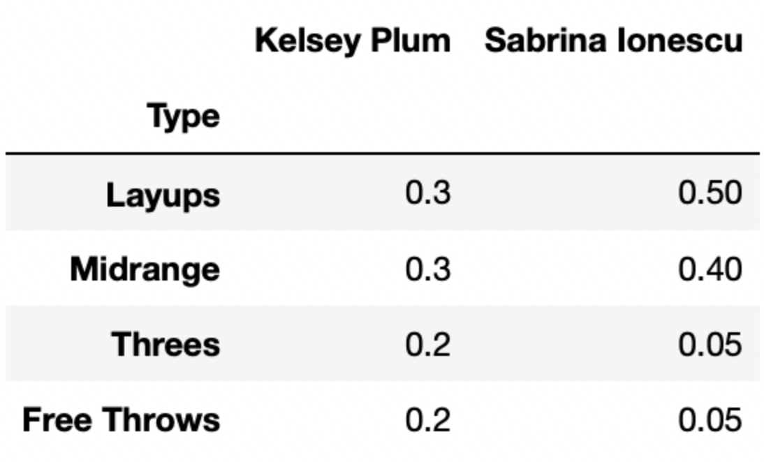
Let’s suppose there are 4 different types of shots a basketball player can take – layups, midrange shots, threes, and free throws.
The DataFrame breakdown has 4 rows and 50 columns – one
row for each of the 4 shot types mentioned above, and one column for
each of 50 different players. Each column of breakdown
describes the distribution of shot types for a single player.
The first few columns of breakdown are shown below.
For instance, 30% of Kelsey Plum’s shots are layups, 30% of her shots are midrange shots, 20% of her shots are threes, and 20% of her shots are free throws.
Below, we’ve drawn an overlaid bar chart showing the shot distributions of Kelsey Plum and Chiney Ogwumike, a player on the Los Angeles Sparks.
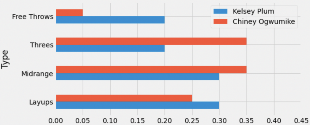
What is the total variation distance (TVD) between Kelsey Plum’s shot distribution and Chiney Ogwumike’s shot distribution? Give your answer as a proportion between 0 and 1 (not a percentage) rounded to three decimal places.
Answer: 0.2
Recall, the TVD is the sum of the absolute differences in proportions, divided by 2. The absolute differences in proportions for each category are as follows:
Then, we have
\text{TVD} = \frac{1}{2} (0.15 + 0.15 + 0.05 + 0.05) = 0.2
The average score on this problem was 84%.
Recall, breakdown has information for 50 different
players. We want to find the player whose shot distribution is the
most similar to Kelsey Plum, i.e. has the lowest TVD
with Kelsey Plum’s shot distribution.
Fill in the blanks below so that most_sim_player
evaluates to the name of the player with the most similar shot
distribution to Kelsey Plum. Assume that the column named
'Kelsey Plum' is the first column in breakdown
(and again that breakdown has 50 columns total).
most_sim_player = ''
lowest_tvd_so_far = __(a)__
other_players = np.array(breakdown.columns).take(__(b)__)
for player in other_players:
    player_tvd = tvd(breakdown.get('Kelsey Plum'),
                     breakdown.get(player))
    if player_tvd < lowest_tvd_so_far:
        lowest_tvd_so_far = player_tvd
__(c)__-1
-0.5
0
0.5
1
np.array([])
''
What goes in blank (b)?
What goes in blank (c)?
Answers: 1, np.arange(1, 50),
most_sim_player = player
Let’s try and understand the code provided to us. It appears that
we’re looping over the names of all other players, each time computing
the TVD between Kelsey Plum’s shot distribution and that player’s shot
distribution. If the TVD calculated in an iteration of the
for-loop (player_tvd) is less than the
previous lowest TVD (lowest_tvd_so_far), the current player
(player) is now the most “similar” to Kelsey Plum, and so
we store their TVD and name (in most_sim_player).
Before the for-loop, we haven’t looked at any other
players, so we don’t have values to store in
most_sim_player and lowest_tvd_so_far. On the
first iteration of the for-loop, both of these values need
to be updated to reflect Kelsey Plum’s similarity with the first player
in other_players. This is because, if we’ve only looked at
one player, that player is the most similar to Kelsey Plum.
most_sim_player is already initialized as an empty string,
and we will specify how to “update” most_sim_player in
blank (c). For blank (a), we need to pick a value of
lowest_tvd_so_far that we can guarantee
will be updated on the first iteration of the for-loop.
Recall, TVDs range from 0 to 1, with 0 meaning “most similar” and 1
meaning “most different”. This means that no matter what, the TVD
between Kelsey Plum’s distribution and the first player’s distribution
will be less than 1*, and so if we initialize
lowest_tvd_so_far to 1 before the for-loop, we
know it will be updated on the first iteration.
lowest_tvd_so_far and
most_sim_player wouldn’t be updated on the first iteration.
Rather, they’d be updated on the first iteration where
player_tvd is strictly less than 1. (We’d expect that the
TVDs between all pairs of players are neither exactly 0 nor exactly 1,
so this is not a practical issue.) To avoid this issue entirely, we
could change if player_tvd < lowest_tvd_so_far to
if player_tvd <= lowest_tvd_so_far, which would make
sure that even if the first TVD is 1, both
lowest_tvd_so_far and most_sim_player are
updated on the first iteration.lowest_tvd_so_far
to a value larger than 1 as well. Suppose we initialized it to 55 (an
arbitrary positive integer). On the first iteration of the
for-loop, player_tvd will be less than 55, and
so lowest_tvd_so_far will be updated.Then, we need other_players to be an array containing
the names of all players other than Kelsey Plum, whose name is stored at
position 0 in breakdown.columns. We are told that there are
50 players total, i.e. that there are 50 columns in
breakdown. We want to take the elements in
breakdown.columns at positions 1, 2, 3, …, 49 (the last
element), and the call to np.arange that generates this
sequence of positions is np.arange(1, 50). (Remember,
np.arange(a, b) does not include the second integer!)
In blank (c), as mentioned in the explanation for blank (a), we need
to update the value of most_sim_player. (Note that we only
arrive at this line if player_tvd is the lowest pairwise
TVD we’ve seen so far.) All this requires is
most_sim_player = player, since player
contains the name of the player who we are looking at in the current
iteration of the for-loop.
The average score on this problem was 70%.
Let’s again consider the shot distributions of Kelsey Plum and Cheney Ogwumike.
We define the maximum squared distance (MSD) between two categorical distributions as the largest squared difference between the proportions of any category.
What is the MSD between Kelsey Plum’s shot distribution and Chiney Ogwumike’s shot distribution? Give your answer as a proportion between 0 and 1 (not a percentage) rounded to three decimal places.
Answer: 0.023
Recall, in the solution to the first subpart of this problem, we calculated the absolute differences between the proportions of each category.
The squared differences between the proportions of each category are computed by squaring the results in the list above (e.g. for Free Throws we’d have (0.05 - 0.2)^2 = 0.15^2). To find the maximum squared difference, then, all we need to do is find the largest of 0.15^2, 0.15^2, 0.05^2, and 0.05^2. Since 0.15 > 0.05, we have that the maximum squared distance is 0.15^2 = 0.0225, which rounds to 0.023.
The average score on this problem was 85%.
For your convenience, we show the first few columns of
breakdown again below.
In basketball:
Suppose that Kelsey Plum is guaranteed to shoot exactly 10 shots a
game. The type of each shot is drawn from the 'Kelsey Plum'
column of breakdown (meaning that, for example, there is a
30% chance each shot is a layup).
Fill in the blanks below to complete the definition of the function
simulate_points, which simulates the number of points
Kelsey Plum scores in a single game. (simulate_points
should return a single number.)
def simulate_points():
    shots = np.random.multinomial(__(a)__, breakdown.get('Kelsey Plum'))
    possible_points = np.array([2, 2, 3, 1])
return __(b)__Answers: 10,
(shots * possible_points).sum()
To simulate the number of points Kelsey Plum scores in a single game, we need to:
To simulate the number of shots she takes of each type, we use
np.random.multinomial. This is because each shot,
independently of all other shots, has a 30% chance of being a layup, a
30% chance of being a midrange, and so on. What goes in blank (a) is the
number of shots she is taking in total; here, that is 10.
shots will be an array of length 4 containing the number of
shots of each type - for instance, shots may be
np.array([3, 4, 2, 1]), which would mean she took 3 layups,
4 midranges, 2 threes, and 1 free throw.
Now that we have shots, we need to factor in how many
points each type of shot is worth. This can be accomplished by
multiplying shots with possible_points, which
was already defined for us. Using the example where shots
is np.array([3, 4, 2, 1]),
shots * possible_points evaluates to
np.array([6, 8, 6, 1]), which would mean she scored 6
points from layups, 8 points from midranges, and so on. Then, to find
the total number of points she scored, we need to compute the sum of
this array, either using the np.sum function or
.sum() method. As such, the two correct answers for blank
(b) are (shots * possible_points).sum() and
np.sum(shots * possible_points).
The average score on this problem was 84%.
True or False: If we call simulate_points() 10,000 times
and plot a histogram of the results, the distribution will look roughly
normal.
True
False
Answer: True
The answer is True because of the Central Limit Theorem. Recall, the
CLT states that no matter what the population distribution looks like,
if you take many repeated samples with replacement, the distribution of
the sample means and sample sums will be roughly normal.
simulate_points() returns the sum of a sample of size 10
drawn with replacement from a population, and so if we generate many
sample sums, the distribution of those sample sums will be roughly
normal.
The distribution we are drawing from is the one below.
| Type | Points | Probability |
|---|---|---|
| Layups | 2 | 0.3 |
| Midrange | 2 | 0.3 |
| Threes | 3 | 0.2 |
| Free Throws | 1 | 0.2 |
The average score on this problem was 78%.
Charlie spends 100 days in each of three California cities (San Diego, San Francisco, and Los Angeles). He records the primary weather for each day in each location. The table below shows these values as proportions. For example, 43 of the 100 days that Charlie spent in San Diego had primarily sunny weather.
| Weather | San Diego | San Francisco | Los Angeles | |
|---|---|---|---|---|
| sunny | 0.43 | 0.51 | 0.34 | |
| partly cloudy | 0.24 | 0.18 | 0.22 | |
| cloudy | 0.22 | 0.15 | 0.26 | |
| rainy | 0.11 | 0.16 | 0.18 |
What is the total variation distance between the San Diego and San Francisco weather distributions? Give your answer as an exact decimal.
Answer: 0.13
The average score on this problem was 74%.
Charlie reconsiders his weather categories and decides to count any “partly cloudy” days as “cloudy” days, thereby combining these two categories into one. If he recalculates the TVD between any pair of cities, what will he find?
The new TVD is less than or equal to the old TVD.
The new TVD is greater than or equal to the old TVD.
The new TVD is equal to the old TVD.
There is not enough information to determine the relationship
Answer: The new TVD is less than or equal to the old TVD.
The average score on this problem was 39%.
The DataFrame flowers contains information on a sample
of flower fields. Each row corresponds to a different flower field. The
"Fertilizer" column contains Boolean values corresponding
to whether each flower field uses fertilizer.
You wonder if it could be the case that flower fields are fertilized at random, with each flower field having an 80% chance of being fertilized, independently of all others. You decide to do a hypothesis test to determine whether this could or could not be the case, testing at the p=0.05 significance level. You will use as your test statistic the absolute difference between 0.8 and the proportion of fertilized flower fields.
Complete the implementation of the function one_stat,
which calculates one simulated value of this test statistic, under the
assumptions of the null hypothesis. Note that the optional argument
p in np.random.choice specifies the
probabilities with which each element is chosen (here, there is a 0.8
probability of selecting True).
def one_stat():
    sample_size = __(a)__
    random_choice = (np.random.choice([True, False],
                     sample_size, p=[0.8, 0.2]))
return __(b)__(a): flowers.shape[0]
(b):
abs(random_choice.sum() / sample_size - 0.8)
The average score on this problem was 59%.
Complete the implementation of the function
one_stat_differently, which also calculates one simulated
value of this test statistic under the null.
def one_stat_differently():
    multi = np.random.multinomial(__(c)__)
return __(d)__(c): flowers.shape[0], [0.8, 0.2]
(d):
abs(multi[0] / flowers.shape[0] - 0.8)
The average score on this problem was 65%.
Fill in the blanks to calculate 10,000 simulated values of the test
statistic and collect them in an array called many_stats.
You can use the functions you’ve already written to help you.
        many_stats = __(e)__
        for i in np.arange(10000):
many_stats = __(f)__(e): np.array([])
(f): np.append(many_stats, one_stat())
The average score on this problem was 75%.
Suppose that the observed value of the test statistic is 0.04. What do we conclude?
Reject the null hypothesis.
Accept the null hypothesis.
Fail to reject the null hypothesis.
Not enough information.
Answer: Not enough information.
The average score on this problem was 15%.
True or False: We could construct a confidence interval to test these hypotheses.
True
False
Answer: True
The average score on this problem was 83%.
Detective Peter asks another staff member, Ray, to write code to run
the permutation test with 10,000 permutations. Ray comes up with his own
test statistic and writes the following code to calculate an observed
statistic, stored in observed_stat. Ray also wrote code
(not shown) to store 10,000 simulated test statistics, each calculated
in a manner matching the code for the observed statistic, in the array
called simulated_stats. Fill in the two blanks below so it
correctly computes the p-value for testing whether Jeffrey is the
harsher grader.
observed_stat = (abs(grading[grading.get('grader') == 'Kate']
    .get('score').mean())
    - abs(grading[grading.get('grader') == 'Jeffrey']
    .get('score').mean()))

p_value = (simulated_stats ___(a)___ observed_stat).sum() / ___(b)___(a)
Answer: >=
The p-value is the proportion of simulated statistics that are at
least as extreme as the observed statistic in the direction consistent
with Ray’s definition of the statistic. With this setup, larger values
correspond to more extreme outcomes in one tail, so we count simulations
with simulated_stats >= observed_stat.
The average score on this problem was 50%.
(b)
Answer: len(simulated_stats)
(equivalently 10000)
The numerator counts how many simulated statistics meet the inequality; dividing by the number of simulations gives the empirical p-value.
The average score on this problem was 79%.