← return to practice.dsc10.com
Below are practice problems tagged for Lecture 22 (rendered directly from the original exam/quiz sources).
We’re now interested in investigating the differences between the masses of Adelie penguins and Chinstrap penguins. Specifically, our null hypothesis is that their masses are drawn from the same population distribution, and any observed differences are due to chance only.
Below, we have a snippet of working code for this hypothesis test,
for a specific test statistic. Assume that adelie_chinstrap
is a DataFrame of only Adelie and Chinstrap penguins, with just two
columns – 'species' and 'mass'.
stats = np.array([])
num_reps = 500
for i in np.arange(num_reps):
    # --- line (a) starts ---
    shuffled = np.random.permutation(adelie_chinstrap.get('species'))
    # --- line (a) ends ---

    # --- line (b) starts ---
    with_shuffled = adelie_chinstrap.assign(species=shuffled)
    # --- line (b) ends ---

    grouped = with_shuffled.groupby('species').mean()

    # --- line (c) starts ---
    stat = grouped.get('mass').iloc[0] - grouped.get('mass').iloc[1]
    # --- line (c) ends ---

stats = np.append(stats, stat)Which of the following statements best describe the procedure above?
This is a standard hypothesis test, and our test statistic is the total variation distance between the distribution of Adelie masses and Chinstrap masses
This is a standard hypothesis test, and our test statistic is the difference between the expected proportion of Adelie penguins and the proportion of Adelie penguins in our resample
This is a permutation test, and our test statistic is the total variation distance between the distribution of Adelie masses and Chinstrap masses
This is a permutation test, and our test statistic is the difference in the mean Adelie mass and mean Chinstrap mass
Answer: This is a permutation test, and our test statistic is the difference in the mean Adelie mass and mean Chinstrap mass (Option 4)
Recall, a permutation test helps us decide whether two random samples
come from the same distribution. This test matches our goal of testing
whether the masses of Adelie penguins and Chinstrap penguins are drawn
from the same population distribution. The code above are also doing
steps of a permutation test. In part (a), it shuffles
'species' and stores the shuffled series to
shuffled. In part (b), it assign the shuffled series of
values to 'species' column. Then, it uses
grouped = with_shuffled.groupby('species').mean() to
calculate the mean of each species. In part (c), it computes the
difference between mean mass of the two species by first getting the
'mass' column and then accessing mean mass of each group
(Adelie and Chinstrap) with positional index 0 and
1.
The average score on this problem was 98%.
Currently, line (c) (marked with a comment) uses .iloc. Which of the following options compute the exact same statistic as line (c) currently does?
Option 1:
stat = grouped.get('mass').loc['Adelie'] - grouped.get('mass').loc['Chinstrap']Option 2:
stat = grouped.get('mass').loc['Chinstrap'] - grouped.get('mass').loc['Adelie']Option 1 only
Option 2 only
Both options
Neither option
Answer: Option 1 only
We use df.get(column_name).iloc[positional_index] to
access the value in a column with positional_index.
Similarly, we use df.get(column_name).loc[index] to access
value in a column with its index. Remember
grouped is a DataFrame that
groupby('species'), so we have species name
'Adelie' and 'Chinstrap' as index for
grouped.
Option 2 is incorrect since it does subtraction in the reverse order
which results in a different stat compared to
line(c). Its output will be -1
\cdot stat. Recall, in
grouped = with_shuffled.groupby('species').mean(), we use
groupby() and since 'species' is a column with
string values, our index will be sorted in alphabetical order. So,
.iloc[0] is 'Adelie' and .iloc[1]
is 'Chinstrap'.
The average score on this problem was 81%.
Is it possible to re-write line (c) in a way that uses
.iloc[0] twice, without any other uses of .loc
or .iloc?
Yes, it’s possible
No, it’s not possible
Answer: Yes, it’s possible
There are multiple ways to achieve this. For instance
stat = grouped.get('mass').iloc[0] - grouped.sort_index(ascending = False).get('mass').iloc[0].
The average score on this problem was 64%.
What would happen if we removed line (a), and replaced
line (b) with
with_shuffled = adelie_chinstrap.sample(adelie_chinstrap.shape[0], replace=False)Select the best answer.
This would still run a valid hypothesis test
This would not run a valid hypothesis test, as all values in the
stats array would be exactly the same
This would not run a valid hypothesis test, even though there would
be several different values in the stats array
This would not run a valid hypothesis test, as it would incorporate information about Gentoo penguins
Answer: This would not run a valid hypothesis test,
as all values in the stats array would be exactly the same
(Option 2)
Recall, DataFrame.sample(n, replace = False) (or
DataFrame.sample(n) since replace = False is
by default) returns a DataFrame by randomly sampling n rows
from the DataFrame, without replacement. Since our n is
adelie_chinstrap.shape[0], and we are sampling without
replacement, we will get the exactly same Dataframe (though the order of
rows may be different but the stats array would be exactly
the same).
The average score on this problem was 87%.
What would happen if we removed line (a), and replaced
line (b) with
with_shuffled = adelie_chinstrap.sample(adelie_chinstrap.shape[0], replace=True)Select the best answer.
This would still run a valid hypothesis test
This would not run a valid hypothesis test, as all values in the
stats array would be exactly the same
This would not run a valid hypothesis test, even though there would
be several different values in the stats array
This would not run a valid hypothesis test, as it would incorporate information about Gentoo penguins
Answer: This would not run a valid hypothesis test,
even though there would be several different values in the
stats array (Option 3)
Recall, DataFrame.sample(n, replace = True) returns a
new DataFrame by randomly sampling n rows from the
DataFrame, with replacement. Since we are sampling with replacement, we
will have a DataFrame which produces a stats array with
some different values. However, recall, the key idea behind a
permutation test is to shuffle the group labels. So, the above code does
not meet this key requirement since we only want to shuffle the
"species" column without changing the size of the two
species. However, the code may change the size of the two species.
The average score on this problem was 66%.
What would happen if we replaced line (a) with
with_shuffled = adelie_chinstrap.assign(
    species=np.random.permutation(adelie_chinstrap.get('species'))
)
and replaced line (b) with
with_shuffled = with_shuffled.assign(
    mass=np.random.permutation(adelie_chinstrap.get('mass'))
)
Select the best answer.
This would still run a valid hypothesis test
This would not run a valid hypothesis test, as all values in the
stats array would be exactly the same
This would not run a valid hypothesis test, even though there would
be several different values in the stats array
This would not run a valid hypothesis test, as it would incorporate information about Gentoo penguins
Answer: This would still run a valid hypothesis test (Option 1)
Our goal for the permutation test is to randomly assign masses to
groups, without changing group sizes. The above code shuffles
'species' and 'mass' columns and assigns them
back to the DataFrame. This fulfills our goal.
The average score on this problem was 81%.
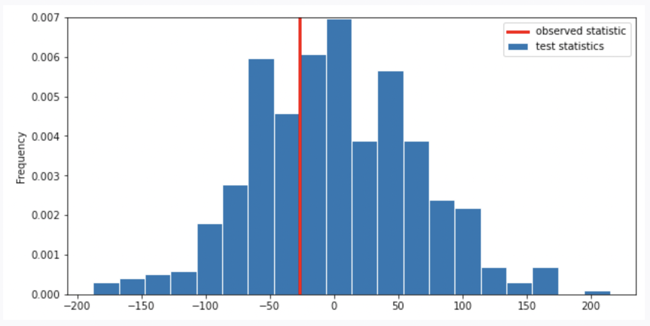
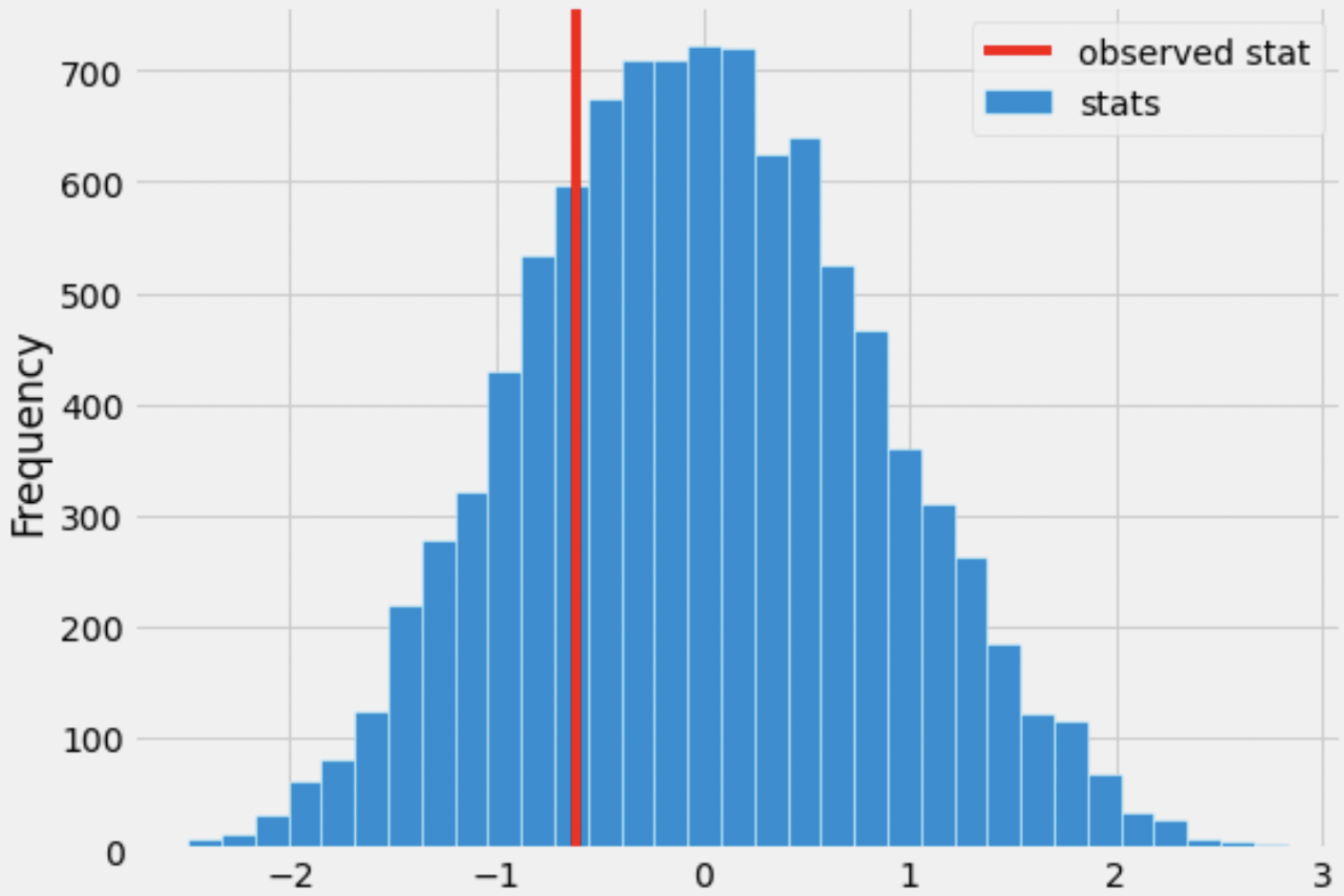
Suppose we run the code for the hypothesis test and see the following empirical distribution for the test statistic. In red is the observed statistic.
Suppose our alternative hypothesis is that Chinstrap penguins weigh more on average than Adelie penguins. Which of the following is closest to the p-value for our hypothesis test?
0
\frac{1}{4}
\frac{1}{3}
\frac{2}{3}
\frac{3}{4}
1
Answer: \frac{1}{3}
Recall, the p-value is the chance, under the null hypothesis, that the test statistic is equal to the value that was observed in the data or is even further in the direction of the alternative. Thus, we compute the proportion of the test statistic that is equal or less than the observed statistic. (It is less than because less than corresponds to the alternative hypothesis “Chinstrap penguins weigh more on average than Adelie penguins”. Recall, when computing the statistic, we use Adelie’s mean mass minus Chinstrap’s mean mass. If Chinstrap’s mean mass is larger, the statistic will be negative, the direction of less than the observed statistic).
Thus, we look at the proportion of area less than or on the red line (which represents observed statistic), it is around \frac{1}{3}.
The average score on this problem was 80%.
In apps, our sample of 1,000 credit card applications,
applicants who were approved for the credit card have fewer dependents,
on average, than applicants who were denied. The mean number of
dependents for approved applicants is 0.98, versus 1.07 for denied
applicants.
To test whether this difference is purely due to random chance, or whether the distributions of the number of dependents for approved and denied applicants are truly different in the population of all credit card applications, we decide to perform a permutation test.
Consider the incomplete code block below.
def shuffle_status(df):
    shuffled_status = np.random.permutation(df.get("status"))
    return df.assign(status=shuffled_status).get(["status", "dependents"])

def test_stat(df):
    grouped = df.groupby("status").mean().get("dependents")
    approved = grouped.loc["approved"]
    denied = grouped.loc["denied"]
    return __(a)__

stats = np.array([])
for i in np.arange(10000):
    shuffled_apps = shuffle_status(apps)
    stat = test_stat(shuffled_apps)
    stats = np.append(stats, stat)

p_value = np.count_nonzero(__(b)__) / 10000
Below are six options for filling in blanks (a) and (b) in the code above.
| Blank (a) | Blank (b) | |
|---|---|---|
| Option 1 | denied - approved |
stats >= test_stat(apps) |
| Option 2 | denied - approved |
stats <= test_stat(apps) |
| Option 3 | approved - denied |
stats >= test_stat(apps) |
| Option 4 | np.abs(denied - approved) |
stats >= test_stat(apps) |
| Option 5 | np.abs(denied - approved) |
stats <= test_stat(apps) |
| Option 6 | np.abs(approved - denied) |
stats >= test_stat(apps) |
The correct way to fill in the blanks depends on how we choose our null and alternative hypotheses.
Suppose we choose the following pair of hypotheses.
Null Hypothesis: In the population, the number of dependents of approved and denied applicants come from the same distribution.
Alternative Hypothesis: In the population, the number of dependents of approved applicants and denied applicants do not come from the same distribution.
Which of the six presented options could correctly fill in blanks (a) and (b) for this pair of hypotheses? Select all that apply.
Option 1
Option 2
Option 3
Option 4
Option 5
Option 6
None of the above.
Answer: Option 4, Option 6
For blank (a), we want to choose a test statistic that helps us
distinguish between the null and alternative hypotheses. The alternative
hypothesis says that denied and approved
should be different, but it doesn’t say which should be larger. Options
1 through 3 therefore won’t work, because high values and low values of
these statistics both point to the alternative hypothesis, and moderate
values point to the null hypothesis. Options 4 through 6 all work
because large values point to the alternative hypothesis, and small
values close to 0 suggest that the null hypothesis should be true.
For blank (b), we want to calculate the p-value in such a way that it
represents the proportion of trials for which the simulated test
statistic was equal to the observed statistic or further in the
direction of the alternative. For all of Options 4 through 6, large
values of the test statistic indicate the alternative, so we need to
calculate the p-value with a >= sign, as in Options 4
and 6.
While Option 3 filled in blank (a) correctly, it did not fill in blank (b) correctly. Options 4 and 6 fill in both blanks correctly.
The average score on this problem was 78%.
Now, suppose we choose the following pair of hypotheses.
Null Hypothesis: In the population, the number of dependents of approved and denied applicants come from the same distribution.
Alternative Hypothesis: In the population, the number of dependents of approved applicants is smaller on average than the number of dependents of denied applicants.
Which of the six presented options could correctly fill in blanks (a) and (b) for this pair of hypotheses? Select all that apply.
Answer: Option 1
As in the previous part, we need to fill blank (a) with a test
statistic such that large values point towards one of the hypotheses and
small values point towards the other. Here, the alterntive hypothesis
suggests that approved should be less than
denied, so we can’t use Options 4 through 6 because these
can only detect whether approved and denied
are not different, not which is larger. Any of Options 1 through 3
should work, however. For Options 1 and 2, large values point towards
the alternative, and for Option 3, small values point towards the
alternative. This means we need to calculate the p-value in blank (b)
with a >= symbol for the test statistic from Options 1
and 2, and a <= symbol for the test statistic from
Option 3. Only Options 1 fills in blank (b) correctly based on the test
statistic used in blank (a).
The average score on this problem was 83%.
Option 6 from the start of this question is repeated below.
| Blank (a) | Blank (b) | |
|---|---|---|
| Option 6 | np.abs(approved - denied) |
stats >= test_stat(apps) |
We want to create a new option, Option 7, that replicates the behavior of Option 6, but with blank (a) filled in as shown:
| Blank (a) | Blank (b) | |
|---|---|---|
| Option 7 | approved - denied |
Which expression below could go in blank (b) so that Option 7 is equivalent to Option 6?
np.abs(stats) >= test_stat(apps)
stats >= np.abs(test_stat(apps))
np.abs(stats) >= np.abs(test_stat(apps))
np.abs(stats >= test_stat(apps))
Answer:
np.abs(stats) >= np.abs(test_stat(apps))
First, we need to understand how Option 6 works. Option 6 produces
large values of the test statistic when approved is very
different from denied, then calculates the p-value as the
proportion of trials for which the simulated test statistic was larger
than the observed statistic. In other words, Option 6 calculates the
proportion of trials in which approved and
denied are more different in a pair of random samples than
they are in the original samples.
For Option 7, the test statistic for a pair of random samples may
come out very large or very small when approved is very
different from denied. Similarly, the observed statistic
may come out very large or very small when approved and
denied are very different in the original samples. We want
to find the proportion of trials in which approved and
denied are more different in a pair of random samples than
they are in the original samples, which means we want the proportion of
trials in which the absolute value of approved - denied in
a pair of random samples is larger than the absolute value of
approved - denied in the original samples.
The average score on this problem was 56%.
In our implementation of this permutation test, we followed the
procedure outlined in lecture to draw new pairs of samples under the
null hypothesis and compute test statistics — that is, we randomly
assigned each row to a group (approved or denied) by shuffling one of
the columns in apps, then computed the test statistic on
this random pair of samples.
Let’s now explore an alternative solution to drawing pairs of samples under the null hypothesis and computing test statistics. Here’s the approach:
"dependents"
column as the new “denied” sample, and the values at the at the bottom
of the resulting "dependents" column as the new “approved”
sample. Note that we don’t necessarily split the DataFrame exactly in
half — the sizes of these new samples depend on the number of “denied”
and “approved” values in the original DataFrame!Once we generate our pair of random samples in this way, we’ll compute the test statistic on the random pair, as usual. Here, we’ll use as our test statistic the difference between the mean number of dependents for denied and approved applicants, in the order denied minus approved.
Fill in the blanks to complete the simulation below.
Hint: np.random.permutation shouldn’t appear
anywhere in your code.
    def shuffle_all(df):
        '''Returns a DataFrame with the same rows as df, but reordered.'''
        return __(a)__

    def fast_stat(df):
        # This function does not and should not contain any randomness.
        denied = np.count_nonzero(df.get("status") == "denied")
        mean_denied = __(b)__.get("dependents").mean()
        mean_approved = __(c)__.get("dependents").mean()
        return mean_denied - mean_approved

    stats = np.array([])
    for i in np.arange(10000):
        stat = fast_stat(shuffle_all(apps))
stats = np.append(stats, stat)Answer: The blanks should be filled in as follows:
df.sample(df.shape[0])df.take(np.arange(denied))df.take(np.arange(denied, df.shape[0]))For blank (a), we are told to return a DataFrame with the same rows
but in a different order. We can use the .sample method for
this question. We want each row of the input DataFrame df
to appear once, so we should sample without replacement, and we should
have has many rows in the output as in df, so our sample
should be of size df.shape[0]. Since sampling without
replacement is the default behavior of .sample, it is
optional to specify replace=False.
The average score on this problem was 59%.
For blank (b), we need to implement the strategy outlined, where
after we shuffle the DataFrame, we use the values at the top of the
DataFrame as our new “denied sample. In a permutation test, the two
random groups we create should have the same sizes as the two original
groups we are given. In this case, the size of the”denied” group in our
original data is stored in the variable denied. So we need
the rows in positions 0, 1, 2, …, denied - 1, which we can
get using df.take(np.arange(denied)).
The average score on this problem was 39%.
For blank (c), we need to get all remaining applicants, who form the
new “approved” sample. We can .take the rows corresponding
to the ones we didn’t put into the “denied” group. That is, the first
applicant who will be put into this group is at position
denied, and we’ll take all applicants from there onwards.
We should therefore fill in blank (c) with
df.take(np.arange(denied, df.shape[0])).
For example, if apps had only 10 rows, 7 of them
corresponding to denied applications, we would shuffle the rows of
apps, then take rows 0, 1, 2, 3, 4, 5, 6 as our new
“denied” sample and rows 7, 8, 9 as our new “approved” sample.
The average score on this problem was 38%.
Choose the best tool to answer each of the following questions. Note the following:
Are incomes of applicants with 2 or fewer dependents drawn randomly from the distribution of incomes of all applicants?
Hypothesis Testing
Permutation Testing
Bootstrapping
Anwser: Hypothesis Testing
This is a question of whether a certain set of incomes (corresponding to applicants with 2 or fewer dependents) are drawn randomly from a certain population (incomes of all applicants). We need to use hypothesis testing to determine whether this model for how samples are drawn from a population seems plausible.
The average score on this problem was 47%.
What is the median income of credit card applicants with 2 or fewer dependents?
Hypothesis Testing
Permutation Testing
Bootstrapping
Anwser: Bootstrapping
The question is looking for an estimate a specific parameter (the median income of applicants with 2 or fewer dependents), so we know boostrapping is the best tool.
The average score on this problem was 88%.
Are credit card applications approved through a random process in which 50% of applications are approved?
Hypothesis Testing
Permutation Testing
Bootstrapping
Anwser: Hypothesis Testing
The question asks about the validity of a model in which applications are approved randomly such that each application has a 50% chance of being approved. To determine whether this model is plausible, we should use a standard hypothesis test to simulate this random process many times and see if the data generated according to this model is consistent with our observed data.
The average score on this problem was 74%.
Is the median income of applicants with 2 or fewer dependents less than the median income of applicants with 3 or more dependents?
Hypothesis Testing
Permutation Testing
Bootstrapping
Anwser: Permutation Testing
Recall, a permutation test helps us decide whether two random samples come from the same distribution. This question is about whether two random samples for different groups of applicants have the same distribution of incomes or whether they don’t because one group’s median incomes is less than the other.
The average score on this problem was 57%.
What is the difference in median income of applicants with 2 or fewer dependents and applicants with 3 or more dependents?
Hypothesis Testing
Permutation Testing
Bootstrapping
Anwser: Bootstrapping
The question at hand is looking for a specific parameter value (the difference in median incomes for two different subsets of the applicants). Since this is a question of estimating an unknown parameter, bootstrapping is the best tool.
The average score on this problem was 63%.
Aathi is a movie enthusiast looking to dive into book-reading. He visits Bill’s Book Bonanza and asks for help from the employee on duty, Matilda.
Matilda has access to the matilda DataFrame of
transactions from her shifts, as well as the bookstore
DataFrame of all books available in the store. She decides to advise
Aathi based on the ratings of books that are popular enough to have been
purchased during her shifts. Unfortunately, matilda does
not contain information about the rating or genre of the books sold. To
fix this, she merges the two DataFrames and keeps only the columns that
she’ll need.
Fill in the blanks in the code below so that the resulting
merged DataFrame has one row for each book in
matilda, and columns representing the genre and rating of
each such book.
merged = (matilda.merge(bookstore, __(a)__, __(b)__)
.get(["genre", "rating"]))left_on = "ISBN"
right_index = True
Since each "ISBN" uniquely identifies a book, we can
merge on that. We use right_index=True because
"ISBN" is the index in bookstore, not a
column. We need to match it with the "ISBN" column in
matilda.
The average score on this problem was 60%.
In this example, matilda and merged have
the same number of rows. Why is this the case? Choose the answer which
is sufficient alone to guarantee the same number of rows.
Because every book in bookstore appears exactly once in
matilda.
Because every book in matilda appears exactly once in
bookstore.
Because matilda has no duplicate rows.
Because bookstore has no duplicate rows.
Because the books in matilda are a subset of the books
in bookstore.
Answer: Because every book in matilda
appears exactly once in bookstore.
Think about the merging process. Imagine we go through each row of
matilda, one row at a time, and look for corresponding rows
that match in bookstore. If each row of
matilda matches with exactly one row of
bookstore, then the merged DataFrame must have the same
number of rows as matilda started with.
The average score on this problem was 53%.
Matilda uses some babypandas operations on the
merged DataFrame to create the DataFrame pictured below,
which she calls top_two.
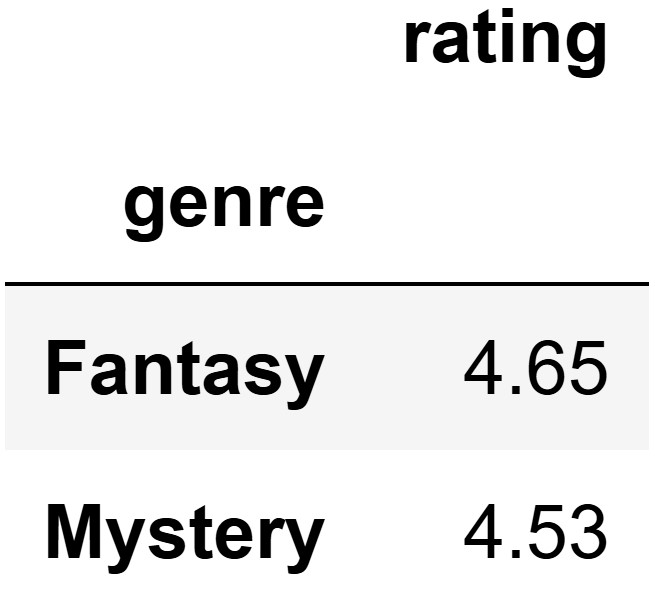
This DataFrame shows the two genres in merged with the
highest mean rating. Note that the "rating" column in
top_two represents a mean rating across many books of the
same genre, not the rating of any individual book.
Write one line of code to define the DataFrame top_two
as described above. It’s okay if you need to write your answer on
multiple lines, as long as it represents one line of code.
Answer:
top_two = merged.groupby("genre").mean().sort_values(by="rating", ascending=False).drop(columns="pages").take([0, 1])
We first groupby the merged DataFrame by
"genre" and calculates the mean rating for each genre. Then
we sort these genres by their average rating in descending order so the
higest rated are at the top. Then, "pages" is dropped since
it’s not needed in our output. Finally, we select the top two genres
with the highest average ratings using .take([0, 1]), which
keeps only the first two rows.
The average score on this problem was 67%.
Based on the data in top_two, Matilda recommends that
Aathi purchase a fantasy book. However, Aathi is skeptical because he
recognizes that the data in merged is only a sample from
the larger population of all transactions at Bill’s Book Bonanza. Before
he makes his purchase, he decides to do a permutation test to determine
whether fantasy books have higher ratings than mystery books in this
larger population.
Select the best statement of the null hypothesis for this permutation test.
Among all books sold at Bill’s Book Bonanza, fantasy books have a higher rating than mystery books, on average.
Among all books sold at Bill’s Book Bonanza, fantasy books do not have a higher rating than mystery books, on average.
Among all books sold at Bill’s Book Bonanza, fantasy books have the same rating as mystery books, on average.
Answer: Among all books sold at Bill’s Book Bonanza, fantasy books have the same rating as mystery books, on average.
The null hypothesis for a permutation test assumes that there is no difference in the population means, implying that fantasy and mystery books have the same average ratings.
The average score on this problem was 62%.
Select the best statement of the alternative hypothesis for this permutation test.
Among all books sold at Bill’s Book Bonanza, fantasy books have a higher rating than mystery books, on average.
Among all books sold at Bill’s Book Bonanza, fantasy books do not have a higher rating than mystery books, on average.
Among all books sold at Bill’s Book Bonanza, fantasy books have the same rating as mystery books, on average.
Answer: Among all books sold at Bill’s Book Bonanza, fantasy books have a higher rating than mystery books, on average.
The alternative hypothesis is that that fantasy books have higher ratings than mystery books, representing the claim being tested against the null hypothesis.
The average score on this problem was 69%.
Aathi decides to use the mean rating for mystery books minus the mean rating for fantasy books as his test statistic. What is his observed value of this statistic?
Answer: -0.12
This comes from subtracting the values provided in the grouped DataFrame in the order mystery minus fantasy: 4.53 - 4.65 = -0.12.
The average score on this problem was 80%.
Which of the following best describes how Aathi will interpret the results of his permutation test?
High values of the observed statistic will make him lean towards the alternative hypothesis.
Low values of the observed statistic will make him lean towards the alternative hypothesis.
Both high and low values of the observed statistic will make him lean towards the alternative hypothesis.
Answer: Low values of the observed statistic will make him lean towards the alternative hypothesis.
Since we are subtracting in the order mystery rating minus fantasy rating, a low (negative) observed statistic would indicate that fantasy books have higher ratings than mystery books. So low values would cause us to reject the null in favor of the alternative.
The average score on this problem was 66%.
Fill in the blanks in the following code to perform Aathi’s permutation test.
just_two = merged[(merged.get("genre") == "Fantasy") |
                  (merged.get("genre") == "Mystery")]

rating_stats = np.array([])
for i in np.arange(10000):
    shuffled = just_two.assign(shuffled = __(a)__)
    grouped = shuffled.groupby("genre").mean().get("shuffled")
    mystery_mean = grouped.iloc[__(b)__]
    fantasy_mean = grouped.iloc[__(c)__]
rating_stats = np.append(rating_stats, mystery_mean - fantasy_mean)np.random.permutation(just_two.get("rating"))We have to permute the "rating" column because of the
code provided on the next line, which groups by genre.
The average score on this problem was 75%.
1It’s important for this question to know that
.groupby("genre") sorts genres alphabetically. In this case, the genre“Fantasy”is before“Mystery”alphabetically,“Mystery”corresponds to the second row (iloc[1]`).
The average score on this problem was 57%.
0 The average score on this problem was 60%.
"Fantasy" is located in the first row, so we use
iloc[0].
Aathi gets a p_value of 0.008, and he will base his purchase on this
result, using the standard p-value cutoff of 0.05. What will Aathi end up doing?
Aathi fails to reject the null hypothesis and will purchase a fantasy book.
Aathi fails to reject the null hypothesis and will purchase a mystery book.
Aathi rejects the null hypothesis and will purchase a fantasy book.
Aathi rejects the null hypothesis and will purchase a mystery book.
Answer: Aathi rejects the null hypothesis and will purchase a fantasy book.
The p-value is lower than our cutoff of 0.05 so we reject the null hypothesis because our observed data doesn’t look like the data we simulated under the assumptions of the null hypothesis.
The average score on this problem was 68%.
Suppose that in movies, the average rating of
"Action" movies is 7.4 and the average rating of
"Horror" movies is 7.2. Based on this data, we decide to
test the following hypotheses:
Null: The ratings of "Action" and
"Horror" movies come from the same distribution.
Alternative: On average, "Action"
movies have a higher rating "Horror" movies.
We’ll use as our test statistic the mean rating of
"Action" movies minus the mean rating of
"Horror" movies.
Fill in the blanks so the code below generates 5000 simulated values of this test statistic and calculates the p-value of our test.
def one_stat(df):
    group_means = df.groupby("New").mean().get("Rating")
    return group_means.loc[__(a)__] - group_mean.loc[__(b)__]

action_horror = movies[(movies.get("Genre") == "Action") |
                       (movies.get("Genre") == "Horror")]
diffs = np.array([])
for i in np.arange(5000):
    new_df = action_horror.assign(New = __(c)__)
    diffs = np.append(diffs, __(d)__)

p_value = np.count_nonzero( __(e)__ ) / 5000"Action""Horror"np.random.permutation(action horror.get("Genre"))one stat(new df)diffs >= 0.2
The average score on this problem was 74%.
Suppose that p_value evaluates to 0.14. Using the standard p-value cutoff of
0.05, which of the two hypotheses is
better supported by the data?
Null
Alternative
Answer: Null
The average score on this problem was 84%.
What kind of hypothesis test did we perform in this question?
Standard hypothesis test
Permutation test
Answer: Permutation test
The average score on this problem was 84%.
Leander conducts a hypothesis test to determine if there is evidence
that players whose batting side is "Left" have higher
"skill" values than those whose batting side is
"Right".
Fill in the blanks to complete the statements of the null and alternative hypotheses.
Null: The mean "skill" of
"Left" batters is ___(a)___ the mean "skill"
of "Right" batters.
Alt: The mean "skill" of
"Left" batters is ___(b)___ the mean "skill"
of "Right" batters.
(a): equal to
(b): greater than
The average score on this problem was 82%.
Select all of the possible test statistics that we could use for this hypothesis test.
The absolute difference in mean "skill" between
"Left" and "Right" batters.
"Left" batters’ maximum "skill" minus
"Right" batters’ maximum "skill".
The TVD between the "skill" distributions for
"Left" and "Right" batters.
None of the above.
Answer: None of the above.
The average score on this problem was 81%.
Fill in the blanks in the code below to perform a permutation test with an appropriate test statistic and compute the p-value.
def get_test_stat(df, column):
    means = df.__(a)__(column).mean().get(__(b)__)
    return means.loc["Left"] - means.loc["Right"]

test_stats = np.array([])
for i in np.arange(5000):
    shuffled_series = np.random.permutation(__(c)__)
    shuffled_df = mlb.assign(shuffled=shuffled_series)
    simulated_test_stat = get_test_stat(__(d)__)
    test_stats = np.append(test_stats, simulated_test_stat)

observed_test_stat = get_test_stat(mlb, "bat")
p_value = np.count_nonzero(__(e)__) / 5000(a): groupby
(b): "skill"
(c): mlb.get("bat")
(d): shuffled df, "shuffled"
(e):
test stats >= observed test stat
The average score on this problem was 67%.
Our test above produces a p-value of 0.038. Select all of the statements below that are true.
At the 0.01 significance level, we fail to reject the null hypothesis.
Using a p-value cutoff of 0.01 results in a test that is 5 times more significant than the test with a p-value cutoff of 0.05.
A p-value is the probability, if the null hypothesis is true, of observing data at least as extreme as what we actually observed.
A p-value of 0.038 means there is a 3.8% chance the null hypothesis is true.
If we used a p-value cutoff of 0.05 and tested many different pairs of hypotheses in which the null hypothesis was actually true, then we would incorrectly reject the null about 5\% of the time.
If we increase the number of repetitions to 10{,}000 the p-value should increase.
If our alternative hypothesis were two-sided instead of one-sided, our p-value would be smaller.
None of the above.
Answer: Options 1, 3, and 5.
The average score on this problem was 89%.
You are browsing the IKEA showroom, deciding whether to purchase the
BILLY bookcase or the LOMMARP bookcase. You are concerned about the
amount of time it will take to assemble your new bookcase, so you look
up the assembly times reported in app_data. Thinking of the
data in app_data as a random sample of all IKEA purchases,
you want to perform a permutation test to test the following
hypotheses.
Null Hypothesis: The assembly time for the BILLY bookcase and the assembly time for the LOMMARP bookcase come from the same distribution.
Alternative Hypothesis: The assembly time for the BILLY bookcase and the assembly time for the LOMMARP bookcase come from different distributions.
Suppose we query app_data to keep only the BILLY
bookcases, then average the 'minutes' column. In addition,
we separately query app_data to keep only the LOMMARP
bookcases, then average the 'minutes' column. If the null
hypothesis is true, which of the following statements about these two
averages is correct?
These two averages are the same.
Any difference between these two averages is due to random chance.
Any difference between these two averages cannot be ascribed to random chance alone.
The difference between these averages is statistically significant.
Answer: Any difference between these two averages is due to random chance.
If the null hypothesis is true, this means that the time recorded in
app_data for each BILLY bookcase is a random number that
comes from some distribution, and the time recorded in
app_data for each LOMMARP bookcase is a random number that
comes from the same distribution. Each assembly time is a
random number, so even if the null hypothesis is true, if we take one
person who assembles a BILLY bookcase and one person who assembles a
LOMMARP bookcase, there is no guarantee that their assembly times will
match. Their assembly times might match, or they might be different,
because assembly time is random. Randomness is the only reason that
their assembly times might be different, as the null hypothesis says
there is no systematic difference in assembly times between the two
bookcases. Specifically, it’s not the case that one typically takes
longer to assemble than the other.
With those points in mind, let’s go through the answer choices.
The first answer choice is incorrect. Just because two sets of
numbers are drawn from the same distribution, the numbers themselves
might be different due to randomness, and the averages might also be
different. Maybe just by chance, the people who assembled the BILLY
bookcases and recorded their times in app_data were slower
on average than the people who assembled LOMMARP bookcases. If the null
hypothesis is true, this difference in average assembly time should be
small, but it very likely exists to some degree.
The second answer choice is correct. If the null hypothesis is true, the only reason for the difference is random chance alone.
The third answer choice is incorrect for the same reason that the second answer choice is correct. If the null hypothesis is true, any difference must be explained by random chance.
The fourth answer choice is incorrect. If there is a difference between the averages, it should be very small and not statistically significant. In other words, if we did a hypothesis test and the null hypothesis was true, we should fail to reject the null.
The average score on this problem was 77%.
For the permutation test, we’ll use as our test statistic the average assembly time for BILLY bookcases minus the average assembly time for LOMMARP bookcases, in minutes.
Complete the code below to generate one simulated value of the test
statistic in a new way, without using
np.random.permutation.
billy = (app_data.get('product') ==
        'BILLY Bookcase, white, 31 1/2x11x79 1/2')
lommarp = (app_data.get('product') ==
          'LOMMARP Bookcase, dark blue-green, 25 5/8x78 3/8')
billy_lommarp = app_data[billy|lommarp]
billy_mean = np.random.choice(billy_lommarp.get('minutes'), billy.sum(), replace=False).mean()
lommarp_mean = _________
billy_mean - lommarp_mean
What goes in the blank?
billy_lommarp[lommarp].get('minutes').mean()
np.random.choice(billy_lommarp.get('minutes'), lommarp.sum(), replace=False).mean()
billy_lommarp.get('minutes').mean() - billy_mean
(billy_lommarp.get('minutes').sum() - billy_mean * billy.sum())/lommarp.sum()
Answer:
(billy_lommarp.get('minutes').sum() - billy_mean * billy.sum())/lommarp.sum()
The first line of code creates a boolean Series with a True value for
every BILLY bookcase, and the second line of code creates the analogous
Series for the LOMMARP bookcase. The third line queries to define a
DataFrame called billy_lommarp containing all products that
are BILLY or LOMMARP bookcases. In other words, this DataFrame contains
a mix of BILLY and LOMMARP bookcases.
From this point, the way we would normally proceed in a permutation
test would be to use np.random.permutation to shuffle one
of the two relevant columns (either 'product' or
'minutes') to create a random pairing of assembly times
with products. Then we would calculate the average of all assembly times
that were randomly assigned to the label BILLY. Similarly, we’d
calculate the average of all assembly times that were randomly assigned
to the label LOMMARP. Then we’d subtract these averages to get one
simulated value of the test statistic. To run the permutation test, we’d
have to repeat this process many times.
In this problem, we need to generate a simulated value of the test
statistic, without randomly shuffling one of the columns. The code
starts us off by defining a variable called billy_mean that
comes from using np.random.choice. There’s a lot going on
here, so let’s break it down. Remember that the first argument to
np.random.choice is a sequence of values to choose from,
and the second is the number of random choices to make. And we set
replace=False, so that no element that has already been
chosen can be chosen again. Here, we’re making our random choices from
the 'minutes' column of billy_lommarp. The
number of choices to make from this collection of values is
billy.sum(), which is the sum of all values in the
billy Series defined in the first line of code. The
billy Series contains True/False values, but in Python,
True counts as 1 and False counts as 0, so billy.sum()
evaluates to the number of True entries in billy, which is
the number of BILLY bookcases recorded in app_data. It
helps to think of the random process like this:
If we think of the random times we draw as being labeled BILLY, then the remaining assembly times still leftover in the bag represent the assembly times randomly labeled LOMMARP. In other words, this is a random association of assembly times to labels (BILLY or LOMMARP), which is the same thing we usually accomplish by shuffling in a permutation test.
From here, we can proceed the same way as usual. First, we need to
calculate the average of all assembly times that were randomly assigned
to the label BILLY. This is done for us and stored in
billy_mean. We also need to calculate the average of all
assembly times that were randomly assigned the label LOMMARP. We’ll call
that lommarp_mean. Thinking of picking times out of a large
bag, this is the average of all the assembly times left in the bag. The
problem is there is no easy way to access the assembly times that were
not picked. We can take advantage of the fact that we can easily
calculate the total assembly time of all BILLY and LOMMARP bookcases
together with billy_lommarp.get('minutes').sum(). Then if
we subtract the total assembly time of all bookcases randomly labeled
BILLY, we’ll be left with the total assembly time of all bookcases
randomly labeled LOMMARP. That is,
billy_lommarp.get('minutes').sum() - billy_mean * billy.sum()
represents the total assembly time of all bookcases randomly labeled
LOMMARP. The count of the number of LOMMARP bookcases is given by
lommarp.sum() so the average is
(billy_lommarp.get('minutes').sum() - billy_mean * billy.sum())/lommarp.sum().
A common wrong answer for this question was the second answer choice,
np.random.choice(billy_lommarp.get('minutes'), lommarp.sum(), replace=False).mean().
This mimics the structure of how billy_mean was defined so
it’s a natural guess. However, this corresponds to the following random
process, which doesn’t associate each assembly with a unique label
(BILLY or LOMMARP):
We could easily get the same assembly time once for BILLY and once for LOMMARP, while other assembly times could get picked for neither. This process doesn’t split the data into two random groups as desired.
The average score on this problem was 12%.
Gabriel is originally from Texas and is trying to convince his friends that Texas has better weather than California. Sophia, who is originally from San Diego, is determined to prove Gabriel wrong.
Coincidentally, both are born in February, so they decide to look at the mean number of sunshine hours of all cities in California and Texas in February. They find that the mean number of sunshine hours for California cities in February is 275, while the mean number of sunshine hours for Texas cities in February is 250. They decide to test the following hypotheses:
Null Hypothesis: The distribution of sunshine hours in February for cities in California and Texas are drawn from the same population distribution.
Alternative Hypothesis: The distribution of sunshine hours in February for cities in California and Texas are not drawn from the same population distribution; rather, California cities see more sunshine hours in February on average than Texas cities.
The test statistic they decide to use is:
\text{mean sunshine hours in California cities – mean sunshine hours in Texas cities}
To simulate data under the null, Sophia proposes the following plan:
Count the number of Texas cities, and call that number
t. Count the total number of cities in both California and
Texas, and call that number n.
Find the total number of sunshine hours across all California and
Texas cities in February, and call that number
total.
Take a random sample of t sunshine hours from the
entire sequence of California and Texas sunshine hours in February in
the dataset. Call this random sample t_samp.
Find the difference between the mean of the values that are not
in t_samp (the California sample) and the mean of the
values that are in t_samp (the Texas sample).
What type of test is this?
Hypothesis test
Permutation test
Answer: Permutation test
Any time we want to decide whether two samples look like they were drawn from the same population distribution, we are conducting a permutation test. In this case, the two samples are (1) the sample of California sunshine hours in February and (2) the sample of Texas sunshine hours in February.
Even though Gabriel and Sophia aren’t “shuffling” the way we normally do when conducting a permutation test, they’re still performing a permutation test. They’re combining the sunshine hours from both states into a single dataset and then randomly reallocating them into two new groups, one representing California and the other Texas, without regard to their original labels.
The average score on this problem was 52%.
Complete the implementation of the function one_stat,
which takes in a DataFrame df that has two columns —
"State", which is either "California" or
"Texas", and "Feb", which contains the number
of sunshine hours in February for each city — and returns a single
simulated test statistic using Sophia’s plan.
    def one_stat(df):
        # You don't need to fill in the ...,
        # assume we've correctly filled them in so that
        # texas_only has only the "Texas" rows from df.
        texas_only = ...
        t = texas_only.shape[0]
        n = df.shape[0]

        total = df.get("Feb").sum()

        t_samp = np.random.choice(df.get("Feb"), t, __(b)__)

        c_mean = __(c)__
        t_mean = t_samp.sum() / t
return c_mean - t_meanWhat goes in blank (b)?
replace=True
replace=False
Answer: replace=False
In order for there to be no overlap between the elements in the Texas sample and California sample, the Texas sample needs to be taken out of the total collection of sunshine hours without replacement.
The average score on this problem was 30%.
What goes in blank (c)? (Hint: Our solution uses 4 of the
variables that are defined before c_mean.)
Answer:
(total - t_samp.sum) / (n - t)
For the c_mean calculation, which represents the mean
sunshine hours for the California cities in the simulation, we need to
subtract the total sunshine hours of the Texas sample
(t_samp.sum()) from the total sunshine hours of both states
(total). This gives us the sum of the California sunshine
hours in the simulation. We then divide this sum by the number of
California cities, which is the total number of cities (n)
minus the number of Texas cities (t), to get the mean
sunshine hours for California cities.
The average score on this problem was 21%.
Fill in the blanks below to accurately complete the provided statement.
“If Sophia and Gabriel want to test the null hypothesis that the mean number of sunshine hours in February in the two states is equal using a different tool, they could use bootstrapping to create a confidence interval for the true value of the test statistic they used in the above test and check whether __(d)__ is in the interval."
What goes in blank (d)? Your answer should be a specific number.
Answer: 0
To conduct a hypothesis test using a confidence interval, our null hypothesis must be of the form “the population parameter is equal to x”; the test is conducted by checking whether x is in the specified interval.
Here, Sophia and Gabriel want to test whether the mean number of sunshine hours in February for the two states is equal; since the confidence interval they created was for the difference in mean sunshine hours, they really want to check whether the difference in mean sunshine hours is 0. (They created a confidence interval for the true value of a - b, and want to test whether a = b; this is the same as testing whether a - b = 0.)
The average score on this problem was 43%.
You want to know if there is a significant difference in the sale
prices of "road" and "hybrid" bikes using a
permutation test. The hypotheses are:
Null: The prices of "road" and
"hybrid" bikes come from the same distribution.
Alt: On average, "hybrid" bikes are
more expensive than "road" bikes.
Using the bikes DataFrame and the difference in group
means (in the order "road" minus "hybrid") as
your test statistic, fill in the blanks so the code below generates
10,000 simulated statistics for the permutation test.
def find_diff(df):
    group_means = df.groupby("shuffled").mean().get("price")
    return group_means.loc["road"] - group_means.loc["hybrid"]

some_bikes = __(x)__
diffs = np.array([])
for i in np.arange(10000):
    shuffled_df = some_bikes.assign(shuffled = __(y)__)
diffs = np.append(diffs, find_diff(shuffled_df))Answer:
(x):
bikes[(bikes.get("style") == "road") | (bikes.get("style") == "hybrid")]
(y): np.random.permutation(some bikes.get("style"))
The average score on this problem was 54%.
Do large values of the observed statistic make us lean towards the null or alternative hypothesis?
Null Hypothesis
Alternative Hypothesis
Answer: Null Hypothesis
The average score on this problem was 63%.
Suppose the p-value for this test evaluates to 0.04. What can you conclude based on this? Select all that apply.
Reject the null hypothesis at a significance level of 0.01.
Fail to reject the null hypothesis at a significance level of 0.01.
Reject the null hypothesis at a significance level of 0.05.
Fail to reject the null hypothesis at a significance level of 0.05
Answer: Fail to reject the null hypothesis at a significance level of 0.01, Reject the null hypothesis at a significance level of 0.05.
The average score on this problem was 48%.
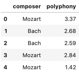
In music theory, polyphony is a number that counts how many independent melodies are being played at the same time. Polyphony is an integer at any given moment, but the average polyphony for a song can be a non-integer.
Minchan collects some data on pieces composed by Johann Sebastian
Bach and Wolfgang Amadeus Mozart. Minchan’s data is in the DataFrame
music, whose first few rows are shown at right. For each
piece, we have the composer and the average polyphony.
Minchan wants to conduct a permutation test with the following hypotheses:
Null Hypothesis: The average polyphony of pieces composed by Bach and the average polyphony of pieces composed by Mozart are drawn from the same distribution.
Alt Hypothesis: The average polyphony of pieces composed by Bach and the average polyphony of pieces composed by Mozart are drawn from different distributions.
For this permutation test, we will use the absolute difference of medians as our test statistic.
Fill in the blanks below to complete the permutation test described
above. Assume observed is the observed test statistic, and
has already been calculated correctly.
total = 0
for i in np.arange(5000):
    shuffled_composer = np.random.permutation(__(a)__)
    shuffled_df = music.assign(shuff=shuffled_composer)
    poly = shuffled_df.groupby(__(b)__).__(c)__.get("polyphony")
    stat = __(d)__
    if stat __(e)__ observed:
        __(f)__
p_value = total / 5000(a): music.get("composer")
(b): "shuff"
(c): median()
(d):
abs(poly.loc["Bach"] - poly.loc["Mozart"]) can be in either
order, can also use iloc[0], iloc[1]
instead
(e): >=
(f): total = total + 1
The average score on this problem was 58%.
The following distributions come from the "polyphony"
column of music:
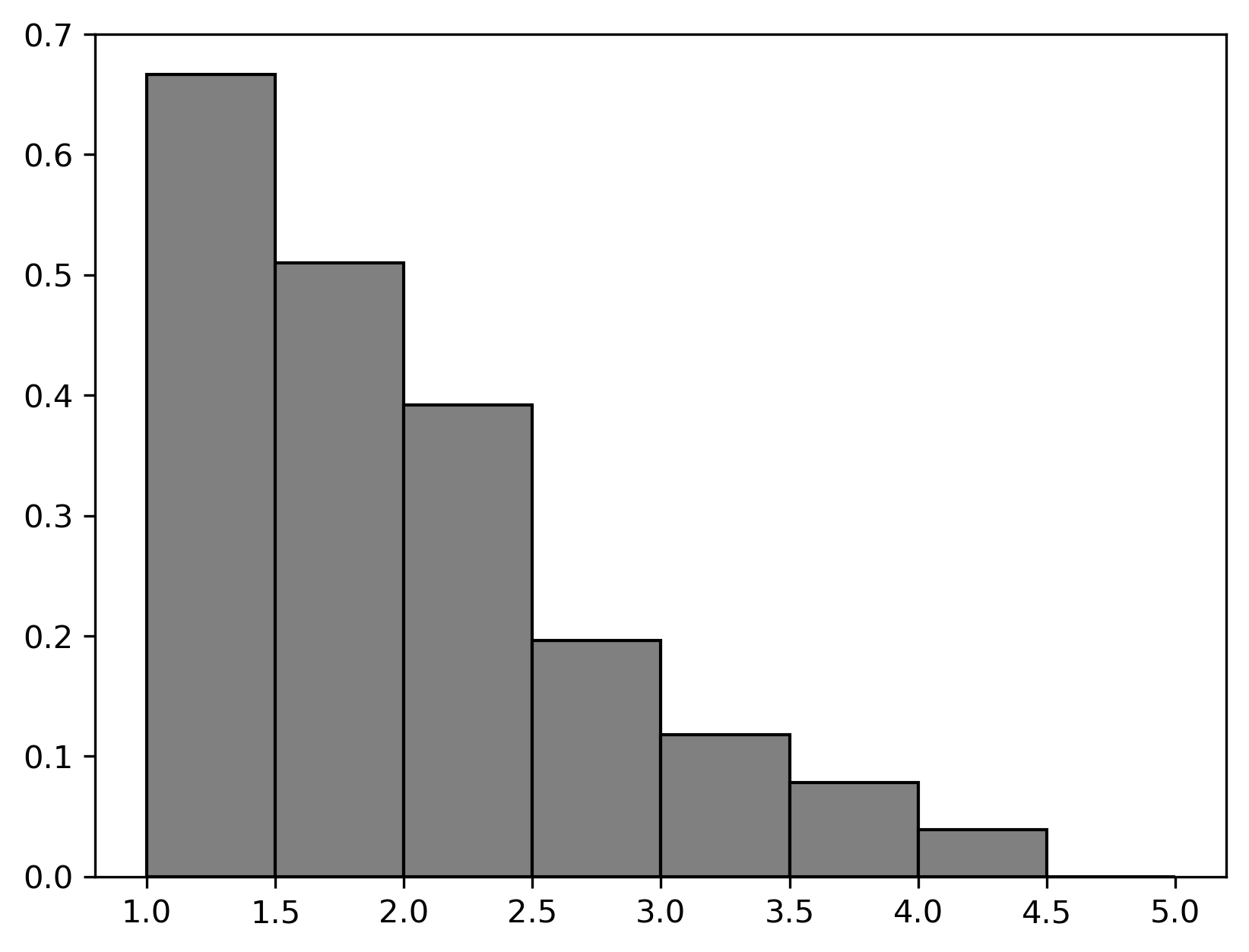
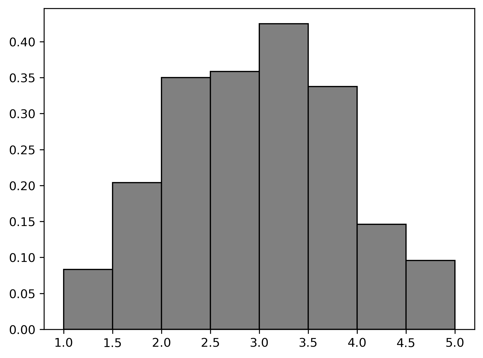
Based on these distributions, estimate the observed value of the test statistic in the permutation test above. Choose the closest answer below.
Answer: 1
The average score on this problem was 51%.
If Minchan repeats the permutation test, this time using the absolute difference of means as the test statistic, how will the observed value of the test statistic change?
The observed value of the test statistic will be smaller than before.
The observed value of the test statistic will be the same as before.
The observed value of the test statistic will be bigger than before.
Answer: Option 1
The average score on this problem was 48%.
Answer the following true/false questions.
Note: This problem is out of scope; it covers material no longer included in the course.
When John Snow took off the handle from the Broad Street pump, the number of cholera deaths decreased. Because of this, he could conclude that cholera was caused by dirty water.
True
False
Answer: False
There are a couple details that the problem fails to convey and that we cannot assume. 1) Do we even know that the pump he removed was the only pump with dirty water? 2) Do we know that people even drank/took water from the Broad Street pump? 3) Do we even know what kinds of people drank from the Broad Street pump? We need to eliminate all confounding factors, otherwise, it might be difficult to identify causality.
The average score on this problem was 91%.
If you get a p-value of 0.009 using a permutation test, you can conclude causality.
True
False
Answer: False
Permutation tests don’t prove causality. Remember, we use the permutation test and calculate a p-value to simply reject a null hypothesis, not to prove the alternative hypothesis.
The average score on this problem was 91%.
df.groupby("kind").mean() will have 5 columns.
True
False
Answer: True
Referring to df at the beginning of the exam, we could
see that 5 of the columns have numerical values as inputs, and thus
df.groupby("kind").mean() will return the mean of these 5
numerical columns
The average score on this problem was 74%.
If the 95% confidence interval for dog price is [650, 900], there is a 95% chance that the population dog price is between $650 and $900.
Answer: False
Recall, what a k% confidence level states is that approximately k% of the time, the intervals you create through this process will contain the true population parameter. In this case, the confidence interval states that approximately 95% of the time, the intervals you create through this process will contain the population dog price. However, it will be false if we state it in the reverse order since our population parameter is already fixed.
The average score on this problem was 66%.
For a given sample, an 90% confidence interval is narrower than a 95% confidence interval.
True
False
Answer: True
The more narrow an interval is, the less confident one is that the intervals one creates will contain the true population parameter.
The average score on this problem was 91%.
If you tried to bootstrap your sample 1,000 times but accidentally sampled without replacement, the standard deviation of your test statistics is always equal to 0.
True
False
Answer: True
Note that bootstrapping form a sample without replacement just means that we’re drawing the same sample over and over again. So the resulting test statistic will be the same between each sample, and thus the std of the test statistic is 0.
The average score on this problem was 86%.
You run a permutation test and store 500 simulated test statistics in
an array called stats. You can construct a 95% confidence
interval by finding the 2.5th and 97.5th percentiles of
stats.
True
False
Answer: False
False, to calculate a 95 percent confidence interval, we use bootstrapping to add variation to our samples.
The average score on this problem was 40%.
The distribution of sample proportions is roughly normal for large samples because of the Central Limit Theorem.
True
False
Answer: True
This is just the definition of Central Limit Theorem.
The average score on this problem was 43%.
Note: This problem is out of scope; it covers material no longer included in the course.
The 20th percentile of the sequence [10, 30, 50, 40, 9, 70] is 30.
True
False
Answer: False
Recall, we find the pth percentile in 4 steps:
Sort the collection in increasing order. [9, 10, 30, 40, 50, 70]
Define h to be p\% of n: h = \frac p{100} \cdot n h = \frac {20}{100} \cdot 6 = 1.2
If h is an integer, define k = h. Otherwise, let k be the smallest integer greater than h. Since h (which is 1.2) is not an integer, so k is 2
Take the kth element of the sorted collection (start counting from 1, not 0). Since 10 has an ordinal rank of 2 in the data set, the 20th percentile value of the data set is 10, not 30.
The average score on this problem was 66%.
Chebyshev’s inequality implies that we can always create a 96% confidence interval from a bootstrap distribution using the mean of the distribution plus or minus 5 standard deviations.
Answer: True
By Chebyshev’s theorem, at least 1 - 1 / z^2 of the data
is within z STD of the mean. Thus at least
1 - 1 / 5^2 = 0.96 of the data is within 5 STD of the
mean.
The average score on this problem was 51%.
Suppose Tiffany has a random sample of dogs. Select the most appropriate technique to answer each of the following questions using Tiffany’s dog sample.
Do small dogs typically live longer than medium and large dogs?
Standard hypothesis test
Permutation test
Bootstrapping
Answer: Option 2: Permutation test.
We have two parameters: dog size and life expectancy. Here if there was no significant statistical difference between the life expectancy of different dog sizes, randomly assigning our sampled life expectancy to each dog should lead us to observe similar observations to the observed statistic. Thus using a permutation test to comapre the two groups makes the most sense. We’re not really trying to estimate a spcecific value so bootstrapping isn’t a good idea here. Also, there’s not really a good way to randomly generate life expectancies so a hypothesis test is not a good idea here.
The average score on this problem was 77%.
Does Tiffany’s sample have an even distribution of dog kinds?
Standard hypothesis test
Permutation test
Bootstrapping
Answer: Option 1: Standard hypothesis test.
We’re not really comparing a variable between two groups, but rather looking at the overall distribution, so Permutation testing wouldn’t work too well here. Again, we’re not really trying to estimate anything here so bootstrapping isn’t a good idea. This leaves us with the Standard Hypothesis Test, which makes sense if we use Total Variation Distance as our test statistic.
The average score on this problem was 51%.
What’s the median weight for herding dogs?
Standard hypothesis test
Permutation test
Bootstrapping
Answer: Option 3: Bootstrapping
Here we’re trying to determine a specific value, which immediately leads us to bootstrapping. The other two tests wouldn’t really make sense in this context.
The average score on this problem was 83%.
Do dogs live longer than 12 years on average?
Standard hypothesis test
Permutation test
Bootstrapping
Answer: Option 3: Bootstrapping
While the wording here might throw us off, we’re really just trying to determine the average life expectancy of dogs, and then see how that compares to 12. This leads us to bootstrapping since we’re trying to determine a specific value. The other two tests wouldn’t really make sense in this context.
The average score on this problem was 43%.
You want to use the data in stages to test the following
hypotheses:
Null Hypothesis: In the Tour de France, the mean distance of flat stages is equal to the mean distance of mountain stages.
Alternative Hypothesis: In the Tour de France, the mean distance of flat stages is less than the mean distance of mountain stages.
For the rest of this problem, assume you have assigned a new column
to stages called class, which categorizes
stages into either flat or mountain
stages.
Which of the following test statistics could be used to test the given hypothesis? Select all that apply.
The mean distance of flat stages divided by the mean distance of mountain stages.
The difference between the mean distance of mountain stages and the mean distance of flat stages.
The absolute difference between the mean distance of flat stages and the mean distance of mountain stages.
One half of the difference between the mean distance of flat stages and the mean distance of mountain stages.
The squared difference between the mean distance of flat stages and the mean distance of mountain stages.
Answer: Option 1, Option 2, and Option 4
A test statistic is a single number we use to test which viewpoint the data better supports. During hypothesis testing, we check whether our observed statistic is a “typical value” in the distribution of the test statistic. The alternative hypothesis indicates “less than” so our test statistic needs to summarize both the magnitude and direction of the difference in the categories.
The average score on this problem was 79%.
Assume that for the rest of the question, we will be using the following test statistic: The difference between the mean distance of flat stages and the mean dis- tance of mountain stages.
Fill in the blanks in the code below so that it correctly conducts a hypothesis test of the given hypotheses and returns the p-value.
def hypothesis_test(stages):
    means = stages.groupby("class").mean().get("Distance")
    observed_stat = means.loc["flat"] - means.loc["mountain"]

    simulated_stats = np.array([])
    for i in np.arange(10000):
        shuffled = stages.assign(shuffled = np.random.__(i)__(stages.get("Distance")))
        shuffled_means = shuffled.groupby("class").mean().get("Distance")
        simulated_stat = (shuffled_means.loc["flat"] - shuffled_means.loc["mountain"])
        simulated_stats = __(ii)__(simulated_stats, simulated_stat)

    p_value = np.__(iii)__(simulated_stats <= observed_stat)
return p_valueAnswer:
permutationnp.appendmeanThe first step in a permutation test simulation is to shuffle the
labels or the values. So since this first line in the for loop is
assigning a column called ‘shuffled’, we know we need to use
np.random.permutation() on the "Distances"
column. The next line gets the new means for each group after shuffling
the values and simulated_stat is the simulated difference
in means. Now we know we want to save this simulated statistic and we
have the simulated_stats array, so we want to use an
np.append in (ii) to save this statistic in the array.
Finally after the simulation is complete, we calculate the p-value using
the array of simulated statistics. The p-value is the probability of
seeing the observed result under the null hypothesis.
simulated_stats <= observed_stat returns an array of 0’s
and 1’s depending on whether each simulated statistic is less than or
equal to the observed statistic. Now, to get the probability of seeing a
result equal to or less than the observed, we can simply take the mean
of this array since the mean of an array of 0’s and 1’s is equivalent to
the probability.
The average score on this problem was 77%.
Indicate whether each of the following code snippets would correctly
calculate simulated_stat inside the for-loop
without errors. Where present, assume the blank (i) has
been filled in correctly.
shuffled = stages.assign(shuffled = np.random.__(i)__(stages.get("Distance")))
shuffled_flat = (shuffled[shuffled.get("class") == "flat"].get("shuffled"))
shuffled_mountain = (shuffled[shuffled.get("class") == "mountain"].get("shuffled"))
simulated_stat = shuffled_flat.mean() - shuffled_mountain.mean()
(i):
This code is correct.
This code is incorrect or errors.
shuffled = stages.assign(shuffled = np.random.__(i)__(stages.get("class")))
shuffled_flat = (shuffled[shuffled.get("shuffled") == "flat"].get("Distance"))
shuffled_mountain = (shuffled[shuffled.get("shuffled") == "mountain"].get("Distance"))
simulated_stat = shuffled_flat.mean() - shuffled_mountain.mean()
(ii):
This code is correct.
This code is incorrect or errors.
shuffled = stages.assign(shuffled = np.random.__(i)__(stages.get("Distance")))
shuffled_means = shuffled.groupby("class").mean()
simulated_stat = (shuffled_means.get("Distance").iloc["flat"] -
                  shuffled_means.get("Distance").iloc["mountain"])
(iii):
This code is correct.
This code is incorrect or errors.
Answer:
shuffled shuffles the distances.
shuffled_flat gets the series of flats with the shuffled
distances and shuffled_mountain gets the series of the
mountains with the shuffled distances. Finally
simulated_stat calculates the mean difference between the
two categories.shuffled shuffles the labels.
shuffled_flat gets the series of the distances with the
shuffled label of “flat” and shuffled_mountain gets the
series of the distances with the shuffled label of “mountain”. Finally,
simulated_stat calculates the mean difference between the
two categories.shuffled shuffles the distances and assigns these
shuffled distances to the column ‘shuffled’.
shuffled_means groups by the label and calculates the means
for each column. However, simulated_stat takes the original
distance columns when calculating the difference in means rather than
the shuffled distances which is located in the ‘shuffled’
column making this answer incorrect.
The average score on this problem was 85%.
Assume that the observed statistic for this hypothesis test was equal to -22.5 km. Given that there are 10,000 simulated test statistics generated in the code above, at least how many of those must be equal to -22.5 km in order for us to reject the null hypothesis at an 0.05 significance level?
500
5000
0
9500
10000
Answer: 0
In order to reject the null hypothesis at the 0.05 significance level, the p-value needs to be below 0.05. In order to calculate the p-value, we find the proportion of simulated test statistics that are equal to or less than the observed value. Note the usage of “must be” in the problem. Since these simulated test statistics can be even less than the observed value, none of them have to be equal to the observed value. Thus, the answer is 0.
The average score on this problem was 30%.
Assume that the code above generated a p-value of 0.03. In the space below, please write your interpretation of this p-value. Your answer should include more than simply “we reject/fail to reject the null hypothesis.”
Answer: There is a 3% chance, assuming the null hypothesis is true, of seeing an observed difference in means less than or equal to -22.5 km.
The p-value is the probability of seeing the observed value or something more extreme under the null hypothesis. Knowing this, in this context, since the p-value is 0.03, this means that there is a 3% chance under the null hypothesis of seeing an observed difference in means equal to or less than -22.5km.
The average score on this problem was 44%.
Choose the best tool to answer each of the following questions. Note the following:
What is the median distance of all Tour de France stages?
Hypothesis Testing
Permutation Testing
Bootstrapping
Central Limit Theorem
Answer: Bootstrapping
Since we want the median distance of all the Tour de France stages, we are not testing anything against a hypothesis at all which rules our hypothesis testing and permutation testing. We use bootstrapping to get samples in lieu of a population. Bootstrapping Tour de France distances will give samples of distances from which we can calculate the median of Tour de France stages.
The average score on this problem was 75%.
Is the distribution of Tour de France stage types from before 1960 the same as after 1960?
Hypothesis Testing
Permutation Testing
Bootstrapping
Central Limit Theorem
Answer: Permutation Testing
We are comparing whether the distributions before 1960 and after 1960 are different which means we want to do permutation testing which tests whether two samples come from the same population distribution.
The average score on this problem was 50%.
Are there an equal number of destinations that start with letters from the first half of the alphabet and destinations that start with letters from the second half of the alphabet?
Hypothesis Testing
Permutation Testing
Bootstrapping
Central Limit Theorem
Answer: Hypothesis Testing
We are testing whether two values (the number of destinations that start with letters from the first half of the alphabet and the destinations that start with letters from the second half of the alphabet) are equal to each other which is an indicator to use a hypothesis test.
The average score on this problem was 50%.
Are mountain stages with destinations in France from before 1970 longer than flat stages with destinations in Belgium from after 2000?
Hypothesis Testing
Permutation Testing
Bootstrapping
Central Limit Theorem
Answer: Permutation Testing
We are comparing two distributions (mountain stages with destinations in France from before 1970 and flat stages with destinations in Belgium from after 2000) and seeing if the first distribution is longer than the second. Since we are comparing distributions, we want to perform a permutation test.
The average score on this problem was 40%.
Give an example of a dataset and a question you would want to answer about that dataset which you could answer by performing a permutation test (also known as an A/B test).
Creative responses that are different than ones we’ve already seen in this class will earn the most credit.
Answer: Responses vary. For this question we looked for creative responses. One good example includes
A dataset about prisoners in the US with the sentence times, race, and crime. Do White people who commit homicide get shorter sentence times than Black people who commit homicide? We can clearly perform an A/B test to compare black and white populations as they correlated to shorter sentence times.
The average score on this problem was 93%.
Consider the definition of the function
diff_in_group_means:
def diff_in_group_means(df, group_col, num_col):
    s = df.groupby(group_col).mean().get(num_col)
return s.loc[False] - s.loc[True]It turns out that Kelsey Plum averages 0.61 more assists in games
that she wins (“winning games”) than in games that she loses (“losing
games”). Fill in the blanks below so that observed_diff
evaluates to -0.61.
observed_diff = diff_in_group_means(plum, __(a)__, __(b)__)What goes in blank (a)?
What goes in blank (b)?
Answers: 'Won', 'AST'
To compute the number of assists Kelsey Plum averages in winning and
losing games, we need to group by 'Won'. Once doing so, and
using the .mean() aggregation method, we need to access
elements in the 'AST' column.
The second argument to diff_in_group_means,
group_col, is the column we’re grouping by, and so blank
(a) must be filled by 'Won'. Then, the second argument,
num_col, must be 'AST'.
Note that after extracting the Series containing the average number
of assists in wins and losses, we are returning the value with the index
False (“loss”) minus the value with the index
True (“win”). So, throughout this problem, keep in mind
that we are computing “losses minus wins”. Since our observation was
that she averaged 0.61 more assists in wins than in losses, it makes
sense that diff_in_group_means(plum, 'Won', 'AST') is -0.61
(rather than +0.61).
The average score on this problem was 94%.
After observing that Kelsey Plum averages more assists in winning games than in losing games, we become interested in conducting a permutation test for the following hypotheses:
To conduct our permutation test, we place the following code in a
for-loop.
won = plum.get('Won')
ast = plum.get('AST')
shuffled = plum.assign(Won_shuffled=np.random.permutation(won)) \
               .assign(AST_shuffled=np.random.permutation(ast))
Which of the following options does not compute a valid simulated test statistic for this permutation test?
diff_in_group_means(shuffled, 'Won', 'AST')
diff_in_group_means(shuffled, 'Won', 'AST_shuffled')
diff_in_group_means(shuffled, 'Won_shuffled, 'AST')
diff_in_group_means(shuffled, 'Won_shuffled, 'AST_shuffled')
More than one of these options do not compute a valid simulated test statistic for this permutation test
Answer:
diff_in_group_means(shuffled, 'Won', 'AST')
As we saw in the previous subpart,
diff_in_group_means(shuffled, 'Won', 'AST') computes the
observed test statistic, which is -0.61. There is no randomness involved
in the observed test statistic; each time we run the line
diff_in_group_means(shuffled, 'Won', 'AST') we will see the
same result, so this cannot be used for simulation.
To perform a permutation test here, we need to simulate under the null by randomly assigning assist counts to groups; here, the groups are “win” and “loss”.
As such, Options 2 through 4 are all valid, and Option 1 is the only invalid one.
The average score on this problem was 68%.
Suppose we generate 10,000 simulated test statistics, using one of
the valid options from Question 4.2. The empirical distribution of test
statistics, with a red line at observed_diff, is shown
below.
Roughly one-quarter of the area of the histogram above is to the left of the red line. What is the correct interpretation of this result?
There is roughly a one quarter probability that Kelsey Plum’s number of assists in winning games and in losing games come from the same distribution.
The significance level of this hypothesis test is roughly a quarter.
Under the assumption that Kelsey Plum’s number of assists in winning games and in losing games come from the same distribution, and that she wins 22 of the 31 games she plays, the chance of her averaging at least 0.61 more assists in wins than losses is roughly a quarter.
Under the assumption that Kelsey Plum’s number of assists in winning games and in losing games come from the same distribution, and that she wins 22 of the 31 games she plays, the chance of her averaging 0.61 more assists in wins than losses is roughly a quarter.
Answer: Under the assumption that Kelsey Plum’s number of assists in winning games and in losing games come from the same distribution, and that she wins 22 of the 31 games she plays, the chance of her averaging at least 0.61 more assists in wins than losses is roughly a quarter. (Option 3)
First, we should note that the area to the left of the red line (a quarter) is the p-value of our hypothesis test. Generally, the p-value is the probability of observing an outcome as or more extreme than the observed, under the assumption that the null hypothesis is true. The direction to look in depends on the alternate hypothesis; here, since our alternative hypothesis is that the number of assists Kelsey Plum makes in winning games is higher on average than in losing games, a “more extreme” outcome is where the assists in winning games are higher than in losing games, i.e. where \text{(assists in wins)} - \text{(assists in losses)} is positive or where \text{(assists in losses)} - \text{(assists in wins)} is negative. As mentioned in the solution to the first subpart, our test statistic is \text{(assists in losses)} - \text{(assists in wins)}, so a more extreme outcome is one where this is negative, i.e. to the left of the observed statistic.
Let’s first rule out the first two options.
Now, the only difference between Options 3 and 4 is the inclusion of “at least” in Option 3. Remember, to compute a p-value we must compute the probability of observing something as or more extreme than the observed, under the null. The “or more” corresponds to “at least” in Option 3. As such, Option 3 is the correct choice.
The average score on this problem was 70%.
True or False: The histogram drawn in the previous subpart is a density histogram.
True
False
Answer: False
The area of a density histogram is 1. The area of the histogram drawn in the previous subpart is much larger than 1. In fact, the area of this histogram is in the hundreds or thousands; you can draw a rectangle stretching from -1 to 1 on the x-axis and 0 to 300 on the y-axis that has area 2 \cdot 300 = 600, and this rectangle is much smaller than the larger histogram.
The average score on this problem was 82%.
We want to create a bootstrapped 95% confidence interval for the
median "Complexity" of all cooperative games, given a
sample of 100 cooperative games.
Suppose coop_sample is a DataFrame containing 100 rows
of games, all of which are cooperative games. We’ll calculate the
endpoints left and right of our bootstrapped
95% confidence interval as follows.
medians = np.array([])
for i in np.arange(10000):
    resample = coop_sample.sample(100, replace=True)
    median = np.median(resample.get("Complexity"))
    medians = np.append(medians, median)
left = np.percentile(medians, 2.5)
right = np.percentile(medians, 97.5)
Now consider the interval defined by the endpoints
left_2 and right_2, calculated as follows.
medians_2 = np.array([])
for i in np.arange(10000):
    shuffle = coop_sample.assign(shuffle=
    np.random.permutation(coop_sample.get("Complexity")))
    resample_2 = shuffle.sample(100, replace=True)
    median_2 = np.median(resample_2.get("shuffle"))
    medians_2 = np.append(medians_2, median_2)
left_2 = np.percentile(medians_2, 2.5)
right_2 = np.percentile(medians_2, 97.5)
Which interval should be wider, [left, right] or
[left_2, right_2]?
[left, right]
[left_2, right_2]
Both about the same.
Answer: Both about the same.
It’s important to understand what each code block above is doing in
order to answer this question. Let’s take a look at the original
medians code. We are sampling from the
coop_sample to create a shuffled coop_sample,
we then get the median of the column “Complexity” and append it to the
medians array. Finally, we find the left and right
percentiles of the medians array.
Now we will look at what medians_2 is doing. It looks
like we are adding a new column called “shuffle” to
coop_sample. The column “shuffle” is a
shuffled version of “Complexity”. Then we are taking the
shuffle DataFrame with the “shuffle” column
and sampling from “shuffle” to randomize it again. Then we
get the median of this shuffled column and find its percentiles.
Essentially, both of these blocks of code are taking the
“Complexity” column, shuffling it, finding the median of
the shuffled column, and then finding the confidence interval. Since it
is being done on the same column and in basically the same way both
intervals [left, right] and [left_2, right_2]
are about the same.
The average score on this problem was 77%.
Choose the best tool to answer each of the following questions. Note the following:
Are strategy games rated higher than non-strategy games?
Hypothesis testing
Permutation testing
Bootstrapping
Answer: Permutation testing
Recall that we use a permutation test when we want to determine if two samples are from the same population. The question is asking if “strategy games” are rated higher than “non-strategy games” meaning we have two samples and want to know if they come from the same or different rating populations.
We would not use hypothesis testing here because we are not trying to quantify how weird a test statistic between strategy games and non-strategy games.
We would not use bootstrapping here because we are not given a single sample that we want to re-sample from.
The average score on this problem was 58%.
What is the mean complexity of all games?
Hypothesis testing
Permutation testing
Bootstrapping
Answer: Bootstrapping
Bootstrapping is the act of resampling from a sample. We use bootstrapping because the original sample looks like the population, so by resampling the sample we are able to quantify our uncertainty of the mean complexity of all games. We can use bootstrapping to approximate the distribution of the sample statistic, which is the mean.
We would not use hypothesis testing here because we do not have the population distribution or a sample to test with.
We would not use permutation testing here because we are not trying to find if two samples are from the same population.
The average score on this problem was 89%.
Are there an equal number of cooperative and non-cooperative games?
Hypothesis testing
Permutation testing
Bootstrapping
Answer: Hypothesis Testing
Recall hypothesis tests quantify how “weird” a result is. We use it when we have a population distribution and one sample and we are trying to see if that sample was drawn from the population. In this instance we are trying to find if there are an equal number of cooperative and non-cooperative games. The population distribution is our DataFrame and we are trying to see if the cooperative games and non-cooperative games in our sample come from the same population.
We would not use permutation testing here because there is no numerical data in the column, and it can be answered by just the column of categories.
We would not use bootstrapping because we are not re-sampling from the sample we are given to find a test statistic.
The average score on this problem was 75%.
Are games with more than one domain more complex than games with one domain?
Hypothesis testing
Permutation testing
Bootstrapping
Answer: Permutation testing
Once again we would use permutation testing to solve this problem because we have two samples: games with more than one domain and games with one domain. We do not know the population distribution.
We would not use hypothesis testing because we were not given a population distribution to test the sample against.
We would not use bootstrapping because we are not re-sampling from the sample to find a test statistic.
The average score on this problem was 72%.
The function perm_test should take three inputs:
df, a DataFrame.labels, a string. The name of a column in df that
contains two distinct values, which signify the groups in a permutation
test.data, a string. The name of a column in df that
contains numerical data.The function should return an array of 1000 simulated differences of group means, under the assumption of the null hypothesis in a permutation test, namely that data in both groups come from the same population.
The smaller of the two group labels should be first in the
subtraction. For example, if the two values in the labels
column are "dice game" and "card game", we
would compute the difference as the mean of the "card game"
group minus the mean of the "dice game" group, because
"card game" comes before "dice game"
alphabetically. Note that groupby orders
the rows in ascending order by default.
An incorrect implementation of perm_test is provided
below.
1 def perm_test(df, labels, data):
2   diffs = np.array([])
3   for i in np.arange(1000):
4       df.assign(shuffled=np.random permutation(df.get(data)))
5       means = df.groupby(labels).mean().get(data)
6       diff = means.iloc[0] - means.iloc[1]
7       diffs = np.append(diffs, diff)
8       return diffs
Three lines of code above are incorrect. Your job is to identify which lines of code are incorrect, and describe briefly in English how you would fix them. You don’t need to explain why the current code is wrong, just how to fix it.
The first line that is incorrect is line number: _______
Explain in one sentence how to change this line. Do not write code.
Answer: Line 4; We need to save this as
df.
Recall that df.assign() does not save the added column
to the original df, which means that we need to save line 4
to a variable called df.
The average score on this problem was 55%.
The second line that is incorrect is line number: _______
Explain in one sentence how to change this line. Do not write code.
Answer: Line 5; We need to get
"shuffled" instead of data.
Recall a permutation test is simulating if samples come from the same
population. This means we need to shuffle the data and use it to see if
that would change our result/view. This means in line 5 we want to use
the shuffled data, so we need to do .get(“shuffled”)
instead of .get(“data”).
The average score on this problem was 50%.
The third line that is incorrect is line number: _______
Explain in one sentence how to change this line. Do not write code.
Answer: Line 8; Move it outside of the
for-loop (unindent).
If we have return inside of the for-loop it
will terminate after it goes through the code once! This means all we
have to do is unindent return, moving it outside of the
for-loop.
The average score on this problem was 67%.
Suppose you’ve fixed all the issues with this function, as you described above. Now, you want to use this corrected function to run a permutation test with the following hypotheses:
For this permutation test, consider a children’s game to be a game
that has "Children’s Games" as part of the
"Domains" column. A dice-rolling game is one that has
"Dice Rolling" as part of the "Mechanics"
column, and a non-dice-rolling game is one that does not have
"Dice Rolling" as part of the "Mechanics"
column.
The DataFrame with_dice is defined as follows.
with_dice = games.assign(isDice = games.get("Mechanics").str.contains("Dice Rolling"))Write one line of code that creates an array called
simulated_diffs containing 1000 simulated differences in
group means for this permutation test. You should call your
perm_test function here!
Answer:
simulated diffs = perm_test(with dice[with dice.get("Domains").str.contains("Children’s Games")], "isDice", "Play Time")The inputs to perm_test, in order, are:
Here, the only relevant information is information on
"Children's Games", so the first argument to
perm_test must be a DataFrame in which the
"Domains" column contains "Children's Games",
as described in the question.
Then, since we’re testing whether the distribution of
"Play Time" is different for dice games and non-dice games,
we know that the column with group labels is "isDice"
(which is defined in the call to .assign that is provided
to us in the question), and the column with numerical information is
"Play Time".
The average score on this problem was 60%.
Suppose we’ve stored the observed value of the test statistic for
this permutation test in the variable obs_diff. Fill in the
blank below to find the p-value for this permutation test.
<
<=
>
>=
Answer: >=
We want to find if the simulated_diffs are more or as
extreme as the obs_diff. To be as or more extreme that
means it needs an equal sign. The other part of this is it cannot be
smaller because then it is not as extreme, which means
the answer must be >=.
The average score on this problem was 57%.
Consider the DataFrame
olympians.drop(columns=["Medal", "Year", "Count"]).
State a question we could answer using the data in this DataFrame and a permutation test.
Answer: There are many possible answers for this question. Some examples: “Are male olympians from Team USA significantly taller than male olympians from other countries?”, “Are olympic swimmers heavier than olympic figure skaters?”, “On average, are male athletes heavier than female athletes?” Any question asking for a difference in a numerical variable across olympians from different categories would work, as long as it is not about the dropped columns.
Recall that a permutation test is basically trying to test if two variables come from the same distribution or if the difference between those two variables are so significant that we can’t possibly say that they’re from the same distribution. In general, this means the question would have to involve the age, height, or weight column because they are numerical data.
The average score on this problem was 80%.
State the null and alternative hypotheses for this permutation test.
Answer: Also many possible answers depending on your answer for the first question.
For example, if our question was “Are olympic swimmers heavier than olympic figure skaters?”, then the null hypothesis could be “Olympic swimmers weigh the same as olympic figure skaters” and the alternative could be “Olympic swimmers weigh more than figure skaters.”
The average score on this problem was 80%.
Suppose the Series s is defined as below. Write an
expression involving s that evaluates to the observed value
of the test statistic, and store the result in
observed.
    s = parking.groupby("Structure").mean().get("Occupancy")
    observed = ______
What goes in the blank?
Answer:
s.loc["Hopkins"] - s.loc["Gilman"]
The average score on this problem was 61%.
In running the permutation test, we need to do a simulation that runs
many times, using a for-loop. What should be the first
thing we do inside the for-loop?
Initialize an empty array to store our results.
Define a variable for the number of repetitions.
Permute one of the columns of parking.
Calculate the difference in group means.
Answer: Permute one of the columns of
parking.
The average score on this problem was 79%.
Suppose we store 5000 simulated test statistics in the array
differences. Choose the appropriate symbol to fill in the
calculation of the p-value below.
p_value = np.count_nonzero(differences ______ observed) / 5000 <
<=
==
!=
>
>=
Answer: <=
The average score on this problem was 65%.
Suppose the p-value of our test is 0.01 and we are testing the hypotheses at the 0.05 significance level. Which hypothesis is better supported by the data?
Null
Alternative
Answer: Alternative
The average score on this problem was 93%.
Professor Severus Snape is rumored to display favoritism toward certain students. Specifically, some believe that he awards more house points to students from wizarding families (those with at least one wizarding parent) than students from muggle families (those without wizarding parents).
To investigate this claim, you will perform a permutation test with these hypotheses:
Null Hypothesis: Snape awards house points independently of a student’s family background (wizarding family vs. muggle family). Any observed difference is due to chance.
Alternative Hypothesis: Snape awards more house points to students from wizarding families, on average.
The DataFrame snape is indexed by "Student"
and contains information on each student’s family background
("Family") and the number of house points awarded by Snape
("Points"). The first few rows of snape are
shown below.
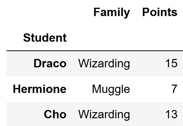
Which of the following is the most appropriate test statistic for our permutation test?
The total number of house points awarded to students from wizarding families minus the total number of house points awarded to students from muggle families.
The mean number of house points awarded to students from wizarding families minus the mean number of house points awarded to students from muggle families.
The number of students from wizarding families minus the number of students from muggle families.
The absolute difference between the mean number of house points awarded to students from wizarding families and the mean number of house points awarded to students from muggle families.
Answer: The mean number of house points awarded to students from wizarding families minus the mean number of house points awarded to students from muggle families.
Let’s look at each of the options:
The average score on this problem was 83%.
Fill in the blanks in the function one_stat, which
calculates one value of the test statistic you chose in part (a), based
on the data in df, which will have columns called
"Family" and "Points".
    def one_stat(df):
        grouped = df.groupby(__(a)__).__(b)__
return __(c)__Answer:
"Family"mean()grouped.get("Points").loc["Wizarding"] - grouped.get("Points").loc["Muggle"]
or
grouped.get("Points").iloc[1] - grouped.get("Points").iloc[0]We first group by the "Family" column, which will create
two groups, one for wizarding families and one for muggle families.
Using mean() as our aggregation function here will give
us the mean of each of our two groups, allowing us to prepare for taking
the difference in group means.
The grouped DataFrame will have two rows with
"Wizarding" and "Muggle" as the index, and
just one column "Points" which contains the mean of each
group. We can either use .loc[] or .iloc[] to
get each group mean, and then take the mean number of house points for
wizarding families minus the mean number of house points for muggle
families. Note that we cannot do this the other way around since our
test statistic we chose in part (a) specifically mentions that
order.
The average score on this problem was 81%.
Fill in the blanks in the function calculate_stats,
which calculates 1000 simulated values of the test statistic you chose
in part (a), under the assumptions of the null hypothesis. As before,
df will have columns called "Family" and
"Points".
    def calculate_stats(df)
        statistics = np.array([])

        for i in np.arange(1000):
            shuffled = df.assign(Points = __(d)__)
            stat = one_stat(__(e)__)
            statistics = __(f)__

return statisticsAnswer:
np.random.permutation(df.get("Points"))shufflednp.append(statistics, stat)Since we performing a permutation test, we need to shuffle the
"Points" column to simulate the null hypothesis, that Snape
awards points independently of family background. Note that shuffling
either "Family" or "Points" would work, but in
this case the code specifies that we are naming this shuffled column
Points.
Next, we pass shuffled into our one_stat
function from part (b) to calculate the test statistic for
shuffled.
We then store our test statistic in the statistics
array, which will have 1000 simulated test statistics under the null
hypothesis once the for loop finishes running.
The average score on this problem was 85%.
Fill in the blanks to calculate the p-value of the permutation test,
based on the data in snape.
    observed = __(g)__
    simulated = __(h)__
p_value = (simulated __(i)__ observed).mean()Answer:
one_stat(snape) or
snape.groupby("Family").mean().get("Points").loc["Wizarding"] - snape.groupby("Family").mean().get("Points").loc["Muggle"]
or
snape.groupby("Family").mean().get("Points").iloc[1] - snape.groupby("Family").mean().get("Points").iloc[0]calculate_stats(snape)>=Our observed is going to be the test statistic we obtain from the
initial observed data. We already created a function to calculate the
test statistic — one_stat—, so we just need to apply it to
our observed data —snape—, giving
one_state(snape) in blank g. You can also manually
calculate the observed test statistic by applying the logic in the
formula giving either:
snape.groupby("Family").mean().get("Points").loc["Wizarding"] - snape.groupby("Family").mean().get("Points").loc["Muggle"]
or
snape.groupby("Family").mean().get("Points").iloc[1] - snape.groupby("Family").mean().get("Points").iloc[0].
The simulated variable is simply the array of simulated test
statistics. We already created a function to run the simulation called
calculate_stats, so we just need to call it with our data
giving calculate_stats(snape) in blank h.
Finally, the p-value is the probability of observing a result as
extreme or even more extreme than our observed. The alternative
hypothesis states that Snape awards more points to students from
wizarding families, and the test statistic is the mean points of
wizarding families minus the mean points from muggle families. Thus, in
this case, a more extreme result, would be the simulated statistics
being larger than the observed value. Thus, we use the
>= operator in blank i to calculate the the number of
simulated statistics that are equal to or greater than the observed
value. Calculating the mean of this boolean series will output this
proportion of seeing a result as extreme or even more extreme than the
observed.
The average score on this problem was 80%.
The average score on this problem was 80%.
The average score on this problem was 81%.
Define mini_snape = snape.take(np.arange(3)) as shown
below.
Determine the value of the following expression.
len(calculate_stats(mini_snape))Answer: 1000
This problem is trying to find the length of the
calculate_stats(snape) array. Looking at
calculate_stats, we know that it calculates a simulated
test statistic and appends it to the output array 1000 times as
indicated in the for loop. Thus, the output of the function is an array
of size 1000.
The average score on this problem was 78%.
With mini_snape defined as above, there will be at most
three unique values in calculate_stats(mini_snape). What
are those three values? Put the smallest value on the left and
the largest on the right.
Answer: -5, -2, and 7
We are trying to find the three unique values outputted by
calculate_stats(mini_snape). The function shuffles the
'Points' column, thus assigning new points to either the
‘Wizarding’ or ‘Muggle’ label. We know that there is one ‘Muggle’ label
and two ‘Wizarding’ labels, so with each iteration, the ‘Wizarding’
label will have two items and the ‘Muggle’ label will only have one
item. There are only three unique values that can be calculated from
this because there are only three unique groups of two and one that can
be made using the data. For example, if the data was A,B,C, then the
only three unique groups of two and one we can create are AC and B, AB
and C, and BC and A. Thus, we can now just run through all the
combinations of groups to find our three unique values. We can do this
by forming each scenario of groupings and calculating the test statistic
by finding the mean number of points for ‘Wizarding’ and then
subtracting by the value of ‘Muggle’ as dictated by the test statistic
(Note: we do not need to take a mean for ‘Muggle’ since there is only
one value assigned here):
Scenario 1:
\begin{align*} \frac{15+7}{2} &= 11 \\ 11 - 13 &= -2 \end{align*}
Scenario 2:
Scenario 3:
\begin{align*} \frac{13+15}{2} &= 14 \\ 14 - 7 &= 7 \end{align*}
Thus, our answer from least to greatest is -5, -2, and 7.
The average score on this problem was 66%.
A researcher collects data on many flowers, some of which have been treated with fertilizer and some of which have not (untreated). The researcher wants to determine whether there is a relationship between fertilizer use and the height of the flowers.
Choose the correct formulation of the null and alternative hypotheses.
Null: There is a difference in the average height of treated and untreated flowers. Alt: There is no difference in the average height of treated and untreated flowers.
Null: There is no difference in the average height
of treated and untreated flowers. Alt: There is a
difference in the average height of treated and untreated flowers.
Null: There is no difference in the average height of treated and untreated flowers. Alt: Treated flowers grow taller,on average, than untreated flowers.
Null: Fertilizer use has no impact on flower height. Alt: Fertilizer use causes taller flowers.
Answer: B
The average score on this problem was 70%.
True or False: We could use a permutation test to test these hypotheses.
True
False
Answer: True
The average score on this problem was 80%.