← return to practice.dsc10.com
Below are practice problems tagged for Lecture 23 (rendered directly from the original exam/quiz sources).
As mentioned in the previous problem, Ashley has sample of 400 rows
of txn. Coincidentally, in Ashley’s sample of 400
transactions, the mean and standard deviation of the
"amount" column both come out to 70 dollars.
Fill in the blank:
“According to Chebyshev’s inequality, at most 25 transactions in
Ashley’s sample
are above ____ dollars; the rest must be below ____ dollars."
What goes in the blank? Give your answer as an integer. Both blanks are filled in with the same number.
Answer: 350
Chebyshev’s inequality says something about how much data falls within a given number of standard deviations. The data that doesn’t fall in that range could be entirely below that range, entirely above that range, or split some below and some above. So the idea is that we should figure out the endpoints of the range for which Chebyshev guarantees that at least 375 transactions must fall. Then at most 25 might fall above that range. So we’ll fill in the blank with the upper limit of that range. Now, since there are 400 transactions, 375 as a proportion becomes \frac{375}{400} = \frac{15}{16}. That’s 1 - \frac{1}{16} or 1 - \left(\frac{1}{4}\right)^2, so we should use z=4 in the statement of Chebyshev’s inequality. That is, \frac{15}{16} proportion of the data falls within 4 standard deviations of the mean. The upper endpoint of that range is 70 (the mean) plus 4 \cdot 70 (four standard deviations), or 5 \cdot 70 = 350.
The average score on this problem was 30%.
Now, we’re given that the mean and standard deviation of the
"lifetime" column in Ashley’s sample are both equal to
c dollars. We’re also given that the
correlation between transaction amounts and lifetime spending in
Ashley’s sample is -\frac{1}{4}.
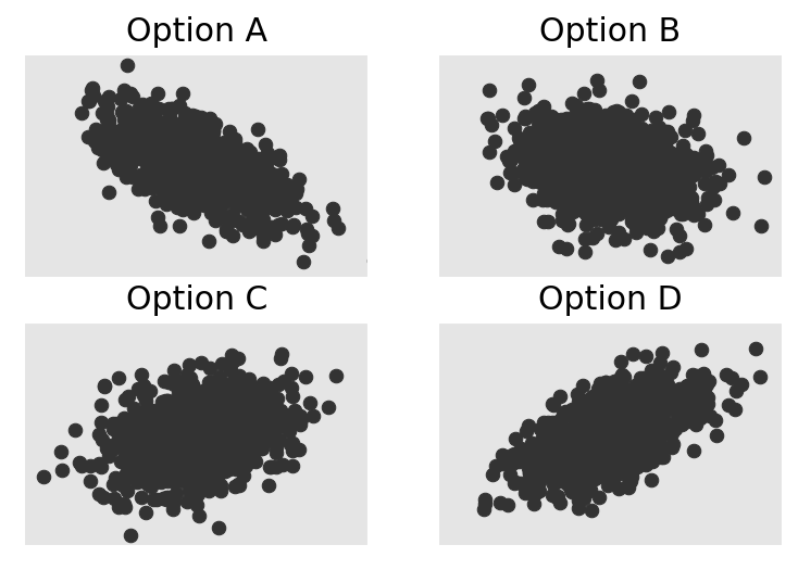
Which of the four options could be a scatter plot of lifetime spending vs. transaction amount?
Option A
Option B
Option C
Option D
Answer: Option B
Here, the main factor which we can use to identify the correct plot is the correlation coefficient. A correlation coefficient of -\frac{1}{4} indicates that the data will have a slight downward trend (values on the y axis will be lower as we go further right). This narrows it down to option A or option B, but option A appears to have too strong of a linear trend. We want the data to look more like a cloud than a line since the correlation is relatively close to zero, which suggests that option B is the more viable choice.
The average score on this problem was 89%.
Ashley decides to use linear regression to predict the lifetime spending of a card given a transaction amount.
The predicted lifetime spending, in dollars, of a card with a transaction amount of 280 dollars is of the form f \cdot c, where f is a fraction. What is the value of f? Give your answer as a simplified fraction.
Answer: f = \frac{1}{4}
This problem requires us to make a prediction using the regression line for a given x = 280. We can solve this problem using original units or standard units. Since 280 is a multiple of 70, and the mean and standard deviation are both 70, it’s pretty straightforward to convert 280 to 3 standard units, as \frac{(280-70)}{70} = \frac{210}{70} = 3. To make a prediction in standard units, all we need to do is multiply by r=-\frac{1}{4}, resulting in a predicted lifetime spending of =-\frac{3}{4} in standard units. Since we are told in the previous subpart that both the mean and standard deviation of lifetime spending are c dollars, then converting to original units gives c + -\frac{3}{4} \cdot c = \frac{1}{4} \cdot c, so f = \frac{1}{4}.
The average score on this problem was 42%.
Suppose the intercept of the regression line, when both transaction amounts and lifetime spending are measured in dollars, is 40. What is the value of c? Give your answer as an integer.
Answer: c = 32
We start with the formulas for the mean and intercept of the regression line, then set the mean and SD of x both to 70, and the mean and SD of y both to c, as well as the intercept b to 40. Then we can solve for c.
\begin{align*} m &= r \cdot \frac{\text{SD of } y}{\text{SD of }x} \\ b &= \text{mean of } y - m \cdot \text{mean of } x \\ m &= -\frac{1}{4} \cdot \frac{c}{70} \\ 40 &= c - (-\frac{1}{4} \cdot \frac{c}{70}) \cdot 70 \\ 40 &= c + \frac{1}{4} c \\ 40 &= \frac{5}{4} c \\ c &= 40 \cdot \frac{4}{5} \\ c &= 32 \end{align*}
The average score on this problem was 45%.
True or False: The slope of the regression line, when both variables are measured in standard units, is never more than 1.
Answer: True
Standard units standardize the data into z scores. When converting to Z scores the scale of both the dependent and independent variables are the same, and consequently, the slope can at most increase by 1. Alternatively, according to the reference sheet, the slope of the regression line, when both variables are measured in standard units, is also equal to the correlation coefficient. And by definition, the correlation coefficient can never be greater than 1 (since you can’t have more than a ‘perfect’ correlation).
The average score on this problem was 93%.
In olympians, "Weight" is measured in
kilograms. There are 2.2 pounds in 1 kilogram. If we converted
"Weight" to pounds instead, which of the following
quantities would increase?
The mean of the "Weight" distribution.
The standard deviation of the "Weight" distribution.
The proportion of "Weight" values within 3 standard
deviations
The correlation between "Height" and
"Weight".
The slope of the regression line predicting "Weight"
from
The slope of the regression line predicting "Height"
from
Answer: Options 1, 2, and 5 are correct.
"Weight", μ being the mean in kg and σ being the standard
deviation in kg. Once we scale everything by 2.2 to convert from
kilograms to pounds, we have that"Weight" within 3 standard deviations of the mean stays the
same. Intuitively this should make sense because we are scaling
everything by the same amount, so the proportion of points that are a
specific number of standard deviations away from the mean should be the
same, since the standard deviation and mean get scaled as well. So,
option 3 is incorrect."Weight"(kg) in standard
units is \frac{x~i~−μ}{σ}. Similar to
option 3, "Weight"(pounds) in standard units is \frac{2.2x_{i}-2.2μ}{2.2σ} = \frac{2.2}{2.2}
\frac{x_{i} \cdot μ}{σ} = \frac{x_{i} \cdot μ}{σ}. Again, notice
that the equation in pounds ends up the exact same as in kilograms. The
same applies for "Height" in standard units. Since none of
the variables change when measured in standard units, r doesn’t change.
So, option 4 is incorrect."Weight" and
the x-axis representing "Height". We expect that the taller
someone is, the heavier they will be. So we can expect a positive
regression line slope between Weight and Height. When we convert Weight
from kg to pounds, we are scaling every value in "Weight",
making their values increase. When we scale the the weight values
(y-values) to become bigger, we are making the regression slope even
steeper, because an increase in Height (x) now corresponds to an even
larger increase in Weight(y). So, option 5 is correct."Weight" on the x-axis and
"Height" on the y-axis. Since we are increasing the values
of "Height", we can imagine stretching the x-axis’ values
without changing the y-values, which makes the line more flat and
therefore decreases the slope. So, option 6 is incorrect. Another
approach to both 5 and 6 is to utilize the correlation coefficient
r, which is equal to the slope times \frac{σ~y~}{σ~x~}. We know that multiplying a
set values by a value greater than one increases the spread of the data
which increases standard deviation. In option 5, "Weight"
is in the y-axis, and increasing the numerator of the fraction \frac{σ~y~}{σ~x~} increases r. In
option 6, "Weight" is in the x-axis, and increasing the
denominator the fraction \frac{σ~y~}{σ~x~} decreases r.
The average score on this problem was 80%.
In Olympic hockey, the number of goals a team scores is linearly associated with the number of shots they attempt. In addition, the number of goals a team scores has a mean of 10 and a standard deviation of 5, whereas the number of attempted shots has a mean of 30 and a standard deviation of 10.
Suppose the regression line to predict the number of goals based on the number of shots predicts that for a game with 20 attempted shots, 6 goals will be scored. What is the correlation between the number of goals and the number of attempted shots? Give your answer as an exact fraction or decimal.
Answer: \frac{4}{5}
Recall that the formula of the regression line in standard units is y_{su}=r \cdot x_{su}. Since we are predicting # of goals from the # of shots, let x_{su} represent # of shots in standard units and y_{su} represent # of goals in standard units. Using the formula for standard units with information in the problem, we find x_{su}=\frac{20-30}{10}=(-1) and y_{su}=\frac{6-10}{5}=(-\frac{4}{5}). Hence, (-\frac{4}{5})=r \cdot (-1) and r=\frac{4}{5}.
The average score on this problem was 74%.
In Olympic baseball, the number of runs a team scores is linearly associated with the number of hits the team gets. The number of runs a team scores has a mean of 8 and a standard deviation of 4, while the number of hits has a mean of 24 and a standard deviation of 6. Consider the regression line that predicts the number of runs scored based on the number of hits.
What is the maximum possible predicted number of runs for a team that gets 27 hits?
What is the correlation coefficient in the case where the predicted number of runs for a team with 25 hits is as large as possible?
Answer: 10
This problem asks about the maximum possible of predicted runs for a team with 27 hits, and the correlation coefficient for the case where the predicted number of runs for a team with 25 hits is maximized. Both of these questions relate to the same concept, so we can answer them both in one fell swoop.
Concept:
The key idea is that the highest correlation coefficient leads to maximum predictions. This is because of a simple fact from lecture: When both x (hits) and y (runs) are converted to standard units,
y_\text{pred} (standard units) = r \cdot x (standard units).
So, the maximum slope in standard units, leading to the highest predictions, is 1, since -1 <= r <= 1. If r were any less than 1, we would be multiplying our x value by a smaller number to get our predicted y value, resulting in lower predictions. In other words,
Max(y_\text{pred}) (standard units) = 1 \cdot x (standard units).
Let’s apply that to answer part 1.
In part 1, we are asked the maximum possible predicted runs for a team with 27 hits. 27 in standard units is:
\dfrac{(27 - 24)}{3} = 0.5,
and the highest value of r (yielding the maximum predictions) is 1. So, we have:
\text{Max}\left(y_\text{pred}\right) \text{(standard units) } = 1 \cdot 0.5
\text{Max}\left(y_\text{pred}\right) \text{(standard units) } = 0.5
Now, we simply need to convert our maximum predicted y in standard units back to its original units, and we have our answer:
y \text{ (standard units)} \cdot \text{SD}_y + \text{Mean}_y = y \text{ (original units)}.
0.5 \cdot 4 + 8 = y \text{ (original units)}
10 = y \text{ (original units)}
So, the maximum number of predicted runs for a team with 27 hits is 10.
The average score on this problem was 63%.
Answer: ii) 1
Part 2 uses the same information as part 1. The value of r that results in the largest predictions of y is 1 (explained above). So, the correlation coefficient for the case where the predicted number of runs for a team with 25 hits is maximized is 1.
The average score on this problem was 67%.