← return to practice.dsc10.com
Below are practice problems tagged for Lecture 25 (rendered directly from the original exam/quiz sources).
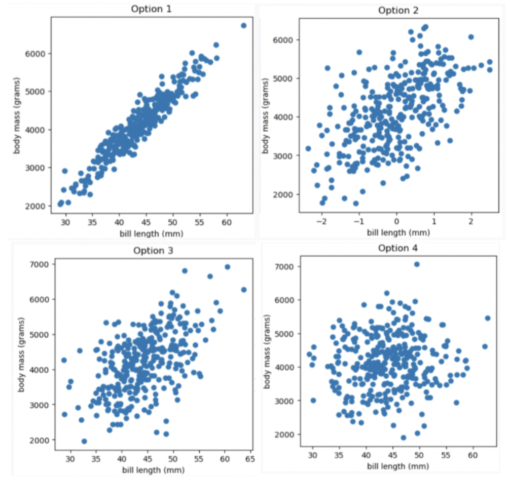
Now let’s study the relationship between a penguin’s bill length (in millimeters) and mass (in grams). Suppose we’re given that
Which of the four scatter plots below describe the relationship between bill length and body mass, based on the information provided in the question?
Option 1
Option 2
Option 3
Option 4
Answer Option 3
Given the correlation coefficient is 0.55, bill length and body mass has a moderate positive correlation. We eliminate Option 1 (strong correlation) and Option 4 (weak correlation).
Given the average bill length is 44 mm, we expect our x-axis to have 44 at the middle, so we eliminate Option 2
The average score on this problem was 91%.
Suppose we want to find the regression line that uses bill length, x, to predict body mass, y. The line is of the form y = mx +\ b. What are m and b?
What is m? Give your answer as a number without any units, rounded to three decimal places.
What is b? Give your answer as a number without units, rounded to three decimal places.
Answer: m = 77, b = 812
m = r \cdot \frac{\text{SD of }y }{\text{SD of }x} = 0.55 \cdot \frac{840}{6} = 77 b = \text{mean of }y - m \cdot \text{mean of }x = 4200-77 \cdot 44 = 812
The average score on this problem was 92%.
What is the predicted body mass (in grams) of a penguin whose bill length is 44 mm? Give your answer as a number without any units, rounded to three decimal places.
Answer: 4200
y = mx\ +\ b = 77 \cdot 44 + 812 = 3388 +812 = 4200
The average score on this problem was 95%.
A particular penguin had a predicted body mass of 6800 grams. What is that penguin’s bill length (in mm)? Give your answer as a number without any units, rounded to three decimal places.
Answer: 77.766
In this question, we want to compute x value given y value y = mx\ +\ b y - b = mx \frac{y - b}{m} = x\ \ \text{(m is nonzero)} x = \frac{y - b}{m} = \frac{6800 - 812}{77} = \frac{5988}{77} \approx 77.766
The average score on this problem was 88%.
Below is the residual plot for our regression line.
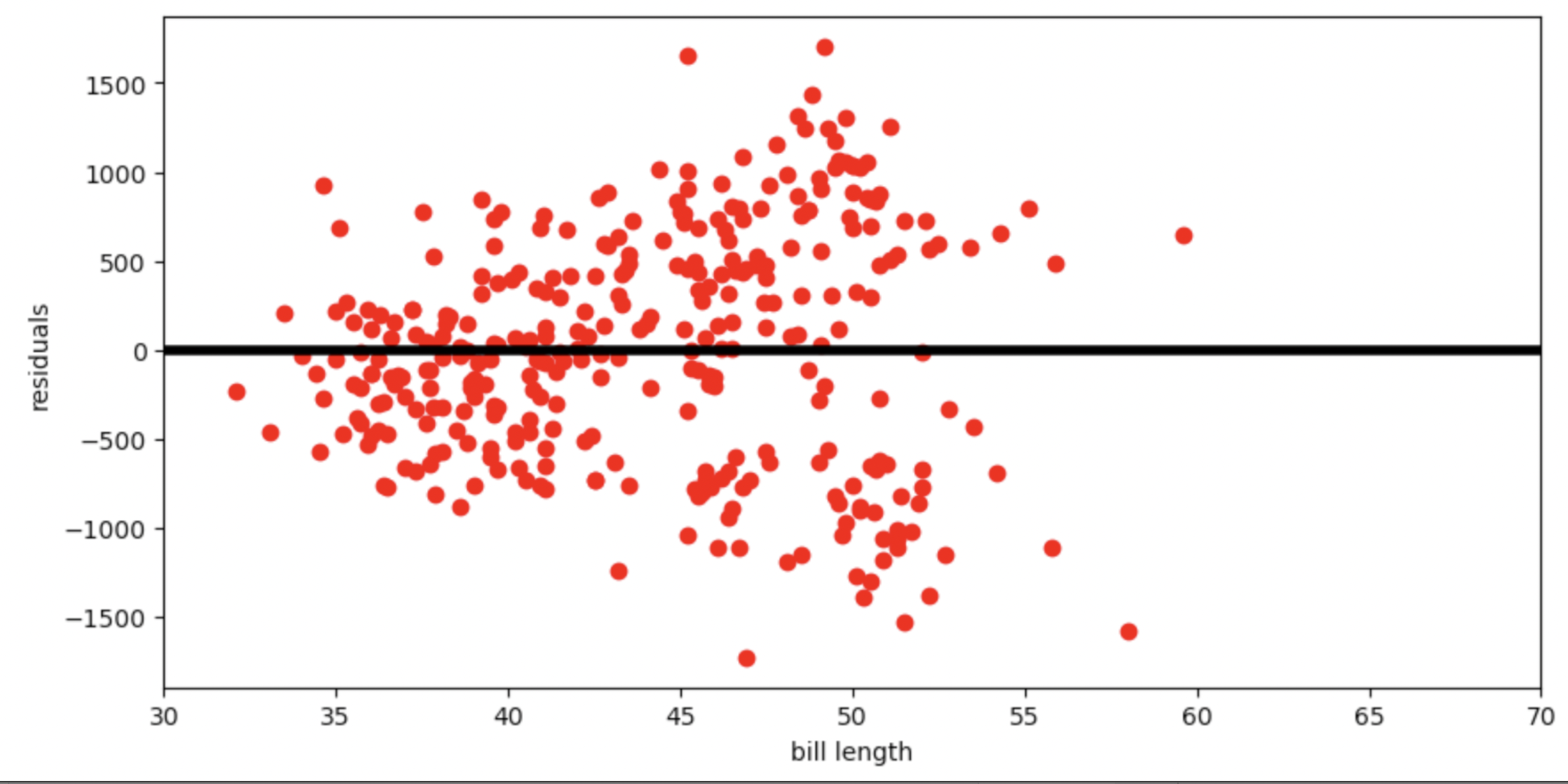
Which of the following is a valid conclusion that we can draw solely from the residual plot above?
For this dataset, there is another line with a lower root mean squared error
The root mean squared error of the regression line is 0
The accuracy of the regression line’s predictions depends on bill length
The relationship between bill length and body mass is likely non-linear
None of the above
Answer: The accuracy of the regression line’s predictions depends on bill length
The vertical spread in this residual plot is uneven, which implies that the regression line’s predictions aren’t equally accurate for all inputs. This doesn’t necessarily mean that fitting a nonlinear curve would be better. It just impacts how we interpret the regression line’s predictions.
The average score on this problem was 40%.
Suppose the price of an IKEA product and the cost to have it assembled are linearly associated with a correlation of 0.8. Product prices have a mean of 140 dollars and a standard deviation of 40 dollars. Assembly costs have a mean of 80 dollars and a standard deviation of 10 dollars. We want to predict the assembly cost of a product based on its price using linear regression.
The NORDMELA 4-drawer dresser sells for 200 dollars. How much do we predict its assembly cost to be?
Answer: 92 dollars
We first use the formulas for the slope, m, and intercept, b, of the regression line to find the equation. For our application, x is the price and y is the assembly cost since we want to predict the assembly cost based on price.
\begin{aligned} m &= r*\frac{\text{SD of }y}{\text{SD of }x} \\ &= 0.8*\frac{10}{40} \\ &= 0.2\\ b &= \text{mean of }y - m*\text{mean of }x \\ &= 80 - 0.2*140 \\ &= 80 - 28 \\ &= 52 \end{aligned}
Now we know the formula of the regression line and we simply plug in x=200 to find the associated y value.
\begin{aligned} y &= mx+b \\ y &= 0.2x+52 \\ &= 0.2*200+52 \\ &= 92 \end{aligned}
The average score on this problem was 76%.
The IDANÄS wardrobe sells for 80 dollars more than the KLIPPAN loveseat, so we expect the IDANÄS wardrobe will have a greater assembly cost than the KLIPPAN loveseat. How much do we predict the difference in assembly costs to be?
Answer: 16 dollars
The slope of a line describes the change in y for each change of 1 in x. The difference in x values for these two products is 80, so the difference in y values is m*80 = 0.2*80 = 16 dollars.
An equivalent way to state this is:
\begin{aligned} m &= \frac{\text{ rise, or change in } y}{\text{ run, or change in } x} \\ 0.2 &= \frac{\text{ rise, or change in } y}{80} \\ 0.2*80 &= \text{ rise, or change in } y \\ 16 &= \text{ rise, or change in } y \end{aligned}
The average score on this problem was 65%.
If we create a 95% prediction interval for the assembly cost of a 100 dollar product and another 95% prediction interval for the assembly cost of a 120 dollar product, which prediction interval will be wider?
The one for the 100 dollar product.
The one for the 120 dollar product.
Answer: The one for the 100 dollar product.
Prediction intervals get wider the further we get from the point (\text{mean of } x, \text{mean of } y) since all regression lines must go through this point. Since the average product price is 140 dollars, the prediction interval will be wider for the 100 dollar product, since it’s the further of 100 and 120 from 140.
The average score on this problem was 45%.
For each IKEA desk, we know the cost of producing the desk, in dollars, and the current sale price of the desk, in dollars. We want to predict sale price based on production cost using linear regression.
For this scenario, which of the following most likely describes the slope of the regression line when both variables are measured in dollars?
less than 0
between 0 and 1, exclusive
more than 1
none of the above (exactly equal to 0 or 1)
Answer: more than 1
The slope of a line represents the change in y for each change of 1 in x. Therefore, the slope of the regression line is the amount we’d predict the sale price to increase when the production cost of an item increases by one dollar. In other words, it’s the sale price per dollar of production cost. This is almost certainly more than 1, otherwise the company would not make a profit. We’d expect that for any company, the sale price of an item should exceed the production cost, meaning the slope of the regression line has a value greater than one.
The average score on this problem was 72%.
For this scenario, which of the following most likely describes the slope of the regression line when both variables are measured in standard units?
less than 0
between 0 and 1, exclusive
more than 1
none of the above (exactly equal to 0 or 1)
Answer: between 0 and 1, exclusive
When both variables are measured in standard units, the slope of the regression line is the correlation coefficient. Recall that correlation coefficients are always between -1 and 1, however, because it’s not realistic for production cost and sale price to be negatively correlated (as that would mean products sell for less if they cost more to produce) we can limit our choice of answer to values between 0 and 1. Because a coefficient of 0 would mean there is no correlation and 1 would mean perfect correlation (that is, plotting the data would create a line), these are unlikely occurrences leaving us with the answer being between 0 and 1, exclusive.
The average score on this problem was 86%.
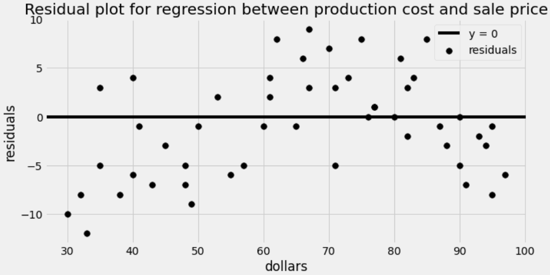
The residual plot for this regression is shown below.
What is being represented on the horizontal axis of the residual plot?
actual production cost
actual sale price
predicted production cost
predicted sale price
Answer: actual production cost
Residual plots show x on the horizontal axis and the residuals, or differences between actual y values and predicted y values, on the vertical axis. Therefore, the horizontal axis here shows the production cost. Note that we are not predicting production costs at all, so production cost means the actual cost to produce a product.
The average score on this problem was 43%.
Which of the following is a correct conclusion based on this residual plot? Select all that apply.
The correlation between production cost and sale price is weak.
It would be better to fit a nonlinear curve.
Our predictions will be more accurate for some inputs than others.
We don’t have enough data to do regression.
The regression line is not the best-fitting line for this data set.
The data set is not representative of the population.
Answer: It would be better to fit a nonlinear curve.
Let’s go through each answer choice.
The correlation between production cost and sale price could be very strong. After all, we are able to predict the sale price within ten dollars almost all the time, since residuals are almost all between -10 and 10.
It would be better to fit a nonlinear curve because the residuals show a pattern. Reading from left to right, they go from mostly negative to mostly positive to mostly negative again. This suggests that a nonlinear curve might be a better fit for our data.
Our predictions are typically within ten dollars of the actual sale price, and this is consistent throughout. We see this on the residual plot by a fairly even vertical spread of dots as we scan from left to right. This data is not heteroscedastic.
We can do regression on a dataset of any size, even a very small data set. Further, this dataset is decently large, since there are a good number of points in the residual plot.
The regression line is always the best-fitting line for any dataset. There may be other curves that are better fits than lines, but when we restrict to lines, the best of the bunch is the regression line.
We have no way of knowing how representative our data set is of the population. This is not something we can discern from a residual plot because such a plot contains no information about the population from which the data was drawn.
The average score on this problem was 61%.
Suppose you know the following information.
apts is
$3,000 with a standard deviation of $400.apts is 2,000
square feet, with a standard deviation of 100 square feet.For all parts of this quesiton, give your answer as an integer.
Suppose the rents are normally distributed. What is the rent below which 84% of apartments are priced?
Answer: $3,400
We can use the 68-95-99.7 rule to approximate this answer. The 68-95-99.7 rule) is a handy shortcut for approximating how much data from a distribution lies below/above/within certain value ranges. It states that, for a normal distribution:
The bottom 84% percent of our apts data is roughly
equivalent to “all data that lies below 1 standard deviation above the
mean.” In this case, let the mean of our distribution be $3,000, and let
the standard deviation be $400; the rent for which 84% of our apartments
are priced is therefore $3,400.
The average score on this problem was 31%.
Sophie’s apartment rents for $5,000. What is this rent in standard units?
Answer: 5
Standard units (or Z-score) is the number of standard deviations an observation is away from the mean of a distribution. In this case, we want to find how many standard deviations ($400) that our observation ($5000) is away from the mean ($3000). The math works out to five standard deviations:
\frac{5000 - 3000}{400} = 5
The average score on this problem was 93%.
Based on what you know about the rent of Sophie’s apartment, use the regression line to predict the square footage of Sophie’s apartment.
Answer: 2450
The correlation coefficient of 0.9 tells us about the slope of the regression line to predict square footage from rent; this means that “for every standard unit traveled right in the x-direction (rent), the regression line heads 0.9 standard units up in the y-direction (square footage).”
Sophie’s apartment rent is $5000 (or five standard units in the x-direction, rent). So, to get our regresion line prediction for the square footage of Sophie’s apartment, we should head 5 \cdot 0.9 = 4.5 standard units upwards from the mean in the y-direction, square footage. The standard deviation for square footage is $100; this implies that the prediction for Sophie’s apartment square footage should be 100 \cdot 4.5 = 450 square feet above the mean (2000 square feet), totaling to a final prediction of 2450 square feet.
The average score on this problem was 66%.
Sophie’s apartment is actually 2,300 square feet. What is the residual of your prediction?
Answer: -150
A residual just measures the difference between the observed and the predicted value. If our observation is 2300 square feet, and our prediction is 2450 square feet, our residual is then -150 square feet.
The average score on this problem was 59%.
Cici’s apartment is 1,800 square feet. Based on this information, use the regression line to predict the rent of Cici’s apartment.
Answer: $2,280
The correlation coefficient of 0.9 also tells us about the slope of the regression line to predict rent from square footage; this means that “for every standard unit traveled right in the x-direction (square footage), the regression line heads 0.9 standard units up in the y-direction (rent).”
Cici’s apartment square footage is 1,800 square feet (or negative two standard units in the x-direction, square footage). So, to get our regresion line prediction for the rent of Cici’s apartment, we should head -2 \cdot 0.9 = -1.8 standard units from the mean in the y-direction, rent. The standard deviation for rent is $400; this implies that the prediction for Cici’s apartment rent should be 400 \cdot -1.8 = 720 square feet below the mean (3000 dollars), totaling to a final prediction of $2280.
The average score on this problem was 23%.
During the Hunger Games, sponsors may purchase supplies for the tributes competing. However, supplies increase in price as the Hunger Games progress. Haymitch collects data on the price, in dollars, of purchasing bread for a tribute over the first 15 days of the Hunger Games competition. He uses linear regression to predict the price of bread based on the day of the competition. His regression line is shown below on a scatterplot of the data.
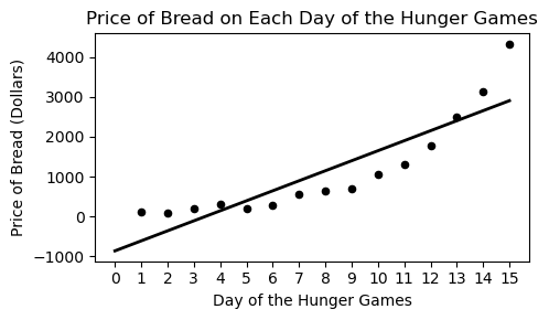
Which of the following plots is the residual plot for the data above?
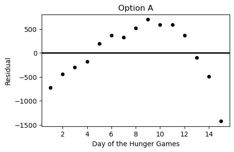
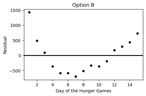
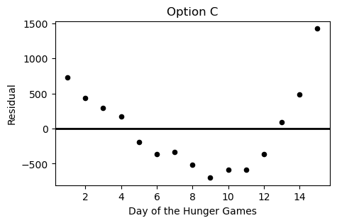
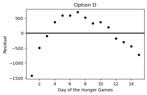
Option A
Option B
Option C
Option D
Answer: Choice C
This choice is correct because the curve in the original scatter plot has a steeper slope at beginning and end, but is actually below the regression line in the middle. This creates positive residuals at the beginning/end and negative residuals in the middle. This eliminates choices A & D. Between choices B & C, we want the negative region of the residual plot ot fall between the fifth and thirteenth days of the hungers games. Only choice C satisfies this.
The average score on this problem was 94%.
What conclusions can Haymitch draw from looking at the residual plot of his regression line? Select all that apply.
The correlation coefficient between these variables is weak (r<0.5).
A line is not the best choice to model the relationship between these variables.
There is a different line that fits the data better than this line.
None of the above.
Answer: Choice 2
The only one of the choices here we can really say for sure is true is Choice B and that is because there is a curved pattern in our residual plot telling us that our straight regression line is missing a trend in the data that a nonlinear model would likely capture. This line of reasoning immidiately also eliminates Choice C, as the curved trend exhibited in the residuals means that no straight line will fit the data better than a nonlinear model. Finally the first choice is also incorrect, because regardless of the trend shown on the residual plot we could still have a strong correlation coefficient.
The average score on this problem was 75%.
Haymitch wants to present the scatter plot to potential sponsors, but he wants to give the prices in thousands of dollars instead of dollars. He divides each of the 15 prices in his data set by 1000, then recalculates the regression line. Which of the following statements are correct? Select all that apply.
The mean of the prices will be divided by 1000.
The standard deviation of the prices will be divided by 1000.
The slope of the regression line predicting price from day will be divided by 1000.
The intercept of the regression line predicting price from day will be divided by 1000.
The slope of the regression line predicting price in standard units from day in standard units will be divided by 1000.
The root mean square error (RMSE) of the regression line will be divided by 1000.
None of the above.
Answer: Choices 1, 2, 3, 4, 6
Choices 1-4 & 6 are correct because when we divide the y variable by 1000, then all of the y variable based quantities will be also scaled down by 1000. This means the mean, std, slope, intercept, and RMSE will all also be scaled down.
Choice 5 is not correct because under standard units, the slope is equal to the correlation coefficient which is resilient to how we scale the units on the graph.
The average score on this problem was 66%.
Sam wants to fit a linear model to predict a dog’s height using its weight.
He first runs the following code:
x = df.get('weight')
y = df.get('height')

def su(vals):
return (vals - vals.mean()) / np.std(vals)Select all of the Python snippets that correctly compute the
correlation coefficient into the variable r.
Snippet 1:
r = (su(x) * su(y)).mean()Snippet 2:
r = su(x * y).mean()Snippet 3:
t = 0
for i in range(len(x)):
    t = t + su(x[i]) * su(y[i])
r = t / len(x)
Snippet 4:
t = np.array([])
for i in range(len(x)):
    t = np.append(t, su(x)[i] * su(y)[i])
r = t.mean()
Snippet 1
Snippet 2
Snippet 3
Snippet 4
Answer: Snippet 1 & 4
Snippet 1: Recall from the reference sheet, the correlation
coefficient is r = (su(x) * su(y)).mean().
Snippet 2: We have to standardize each variable separately so this snippet doesn’t work.
Snippet 3: Note that for this snippet we’re standardizing each
data point within each variable separately, and so we’re not really
standardizing the entire variable correctly. In other words, applying
su(x[i]) to a singular data point is just going to convert
this data point to zero, since we’re only inputting one data point into
su().
Snippet 4: Note that this code is just the same as Snippet 1, except we’re now directly computing the product of each corresponding data points individually. Hence this Snippet works.
The average score on this problem was 81%.
Sam computes the following statistics for his sample:
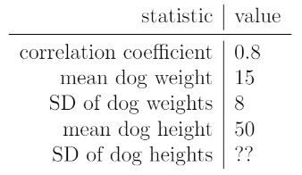
The best-fit line predicts that a dog with a weight of 10 kg has a height of 45 cm.
What is the SD of dog heights?
2
4.5
10
25
45
None of the above
Answer: Option 3: 10
The best fit line in original units are given by
y = mx + b where m = r * (SD of y) / (SD of x)
and b = (mean of y) - m * (mean of x) (refer to reference
sheet). Let c be the STD of y, which we’re trying to find,
then our best fit line is now y = (0.8*c/8)x +
(50-(0.8*c/8)*15). Plugging the two values they gave us into our
best fit line and simplifying gives 45 =
0.1*c*10 + (50 - 1.5*c) which simplifies to 45 = 50 - 0.5*c which gives us an answer of
c = 10.
The average score on this problem was 89%.
Assume that the statistics in part b) still hold. Select all of the statements below that are true. (You don’t need to finish part b) in order to solve this question.)
The relationship between dog weight and height is linear.
The root mean squared error of the best-fit line is smaller than 5.
The best-fit line predicts that a dog that weighs 15 kg will be 50 cm tall.
The best-fit line predicts that a dog that weighs 10 kg will be shorter than 50 cm.
Answer: Option 3 & 4
Option 1: We cannot determine whether two variables are linear simply from a line of best fit. The line of best fit just happens to find the best linear relationship between two varaibles, not whether or not the variables have a linear relationship.
Option 2: To calculate the root mean squared error, we need the actual data points so we can calculate residual values. Seeing that we don’t have access to the data points, we cannot say that the root mean squared error of the best-fit line is smaller than 5.
Option 3: This is true accrding to the problem statement given in part b
Option 4: This is true since we expect there to be a positive correlation between dog height and weight. So dogs that are lighter will also most likely be shorter. (ie a dog that is lighter than 15 kg will most likely be shorter than 50cm)
The average score on this problem was 72%.
Let’s switch our attention to the relationship between the number of
points per game and the number of assists per game for all players in
season. Using season, we compute the following
information:
Let’s start by using points per game (x) to predict assists per game (y).
Tina Charles had 27 points per game in 2021, the most of any player in the WNBA. What is her predicted assists per game, according to the regression line? Round your answer to 3 decimal places.
Answer: 5.4
We need to find and use the regression line to find the predicted y for an x of 27. There are two ways to proceed:
Both solutions work; for the sake of completeness, we’ll show both. Recall, r is the correlation coefficient between x and y, which we are told is 0.65.
Solution 1:
First, we need to convert 27 points per game to standard units. Doing so yields
x_{\text{su}} = \frac{x - \text{mean of }x}{\text{SD of }x} = \frac{27 - 7}{5} = 4
Per the regression line, y_\text{su} = r \cdot x_\text{su}, we have y_\text{su} = 0.65 \cdot 4 = 2.6, which is Tina Charles’ predicted assists per game in standard units. All that’s left is to convert this value back to original units:
\begin{aligned} y_{\text{su}} &= \frac{y - \text{mean of }y}{\text{SD of }y} \\ 2.6 &= \frac{y - 1.5}{1.5} \\ 2.6 \cdot 1.5 + 1.5 &= y \\ y &= \boxed{5.4} \end{aligned}
So, the regression line predicts Tina Charles will have 5.4 assists per game (in original units).
Solution 2:
First, we need to find the slope m and intercept b:
m = r \cdot \frac{\text{SD of }y }{\text{SD of }x} = 0.65 \cdot \frac{1.5}{5} = 0.195
b = \text{mean of }y - m \cdot \text{mean of }x = 1.5 - 0.195 \cdot 7 = 0.135
Then,
y = mx + b \implies y = 0.195 \cdot 27 + 0.135 = \boxed{5.4}
So, once again, the regression line predicts Tina Charles will have 5.4 assists per game.
Note: The numbers in this problem may seem ugly, but students taking this exam had access to calculators since this exam was online. It also turns out that the numbers were easier to work with in Solution 1 over Solution 2; this was intentional.
The average score on this problem was 81%.
Tina Charles actually had 2.1 assists per game in the 2021 season.
What is the error, or residual, for the prediction in the previous subpart? Round your answer to 3 decimal places.
Answer: -3.3
Residuals are defined as follows:
\text{residual} = \text{actual } y - \text{predicted }y
2.1 - 5.4 = -3.3, which gives us our answer.
Note: Many students answered 3.3. Pay attention to the order of the calculation!
The average score on this problem was 82%.
Select all true statements below regarding the regression line between points per game (x) and assists per game (y).
The point (0, 0) is guaranteed to be on the regression line when both x and y are in standard units.
The point (0, 0) is guaranteed to be on the regression line when both x and y are in original units.
The point (7, 1.5) is guaranteed to be on the regression line when both x and y are in standard units.
The point (7, 1.5) is guaranteed to be on the regression line when both x and y are in original units.
None of the above
Answers:
The main idea being assessed here is the fact that the point (\text{mean of }x, \text{mean of }y) always lies on the regression line. Indeed, in original units, 7 is the average x (PPG) and 1.5 is the average y (APG); this information was provided to us at the start of the problem. The nuance behind this problem lies in the units that are being used in the regression line.
When the regression line is in standard units:
When the regression line is in original units:
y = mx + b = mx + \text{mean of }y - m \cdot \text{mean of }x
The average score on this problem was 87%.
So far, we’ve been using points per game (x) to predict assists per game (y). Suppose we found the regression line (when both x and y are in original units) to be y = ax + b.
Now, let’s reverse x and y. That is, we will now use assists per game (x) to predict points per game (y). The resulting regression line (when both x and y are in original units) is y = cx + d.
Which of the following statements is guaranteed to be true?
a = c
a > c
a < c
Using just the information given in this problem, it is impossible to determine the relationship between a and c.
Answer: a < c
The formula for the slope of the regression line is m = r \cdot \frac{\text{SD of }y}{\text{SD of }x}. Note that the correlation coefficient r is symmetric, meaning that the correlation between x and y is the same as the correlation between y and x.
In the two regression lines mentioned in this problem, we have
\begin{aligned} a &= r \cdot \frac{\text{SD of assists per game}}{\text{SD of points per game}} \\ c &= r \cdot \frac{\text{SD of points per game}}{\text{SD of assists per game}} \end{aligned}
We’re told in the problem that the SD of points per game is 5 and the SD of assists per game is 1.5. So, a = r \cdot \frac{1.5}{5} and c = r \cdot \frac{5}{1.5}; since \frac{1.5}{5} < \frac{5}{1.5}, a < c.
The average score on this problem was 74%.
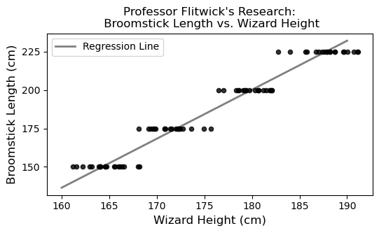
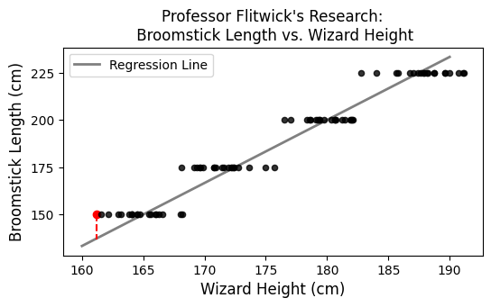
Professor Filius Flitwick is conducting a study whose results will be used to help new Hogwarts students select appropriately sized broomsticks for their flying lessons. Professor Flitwick measures several wizards’ heights and broomstick lengths, both in centimeters. Since broomsticks can only be purchases in specific lengths, the scatterplot of broomstick length vs. height has a pattern of horizontal stripes:
If we group the wizards in Professor Flitwick’s research study by their broomstick length, and average the heights of the wizards in each group, we get the following results.
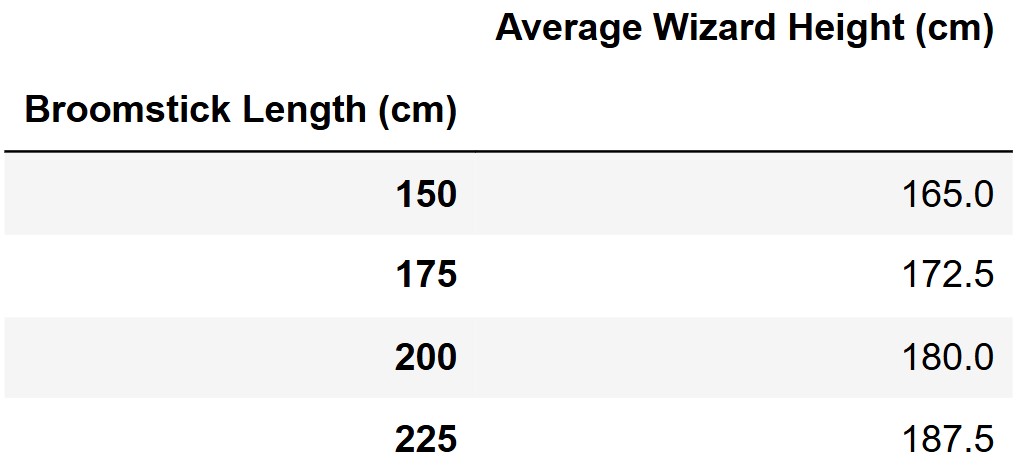
It turns out that the regression line that predicts broomstick length (y) based on wizard height (x) passes through the four points representing the means of each group. For example, the first row of the DataFrame above means that (165, 150) is a point on the regression line, as you can see in the scatterplot.
Based only on the fact that the regression line goes through these points, which of the following could represent the relationship between the standard deviation of broomstick length (y) and wizard height (x)? Select all that apply.
SD(y) = SD(x)
SD(y) = 2\cdot SD(x)
SD(y) = 3\cdot SD(x)
SD(y) = 4\cdot SD(x)
SD(y) = 5\cdot SD(x)
Answer: Options 4 and 5.
To solve this problem, we use the relationship between the slope of the regression line, the correlation coefficient r, and the standard deviations:
\text{slope} = r \cdot \frac{\text{SD}(y)}{\text{SD}(x)}
From the mean points given, we can calculate the slope:
\frac{225 - 150}{187.5 - 165.0} = \frac{75}{22.5} = \frac{10}{3}
We set up the equation:
r \cdot \frac{\text{SD}(y)}{\text{SD}(x)} = \frac{10}{3}
Now consider each option:
If \text{SD}(y) = \text{SD}(x): r = \frac{10}{3} \text{(not valid, since } r > 1\text{)}
If \text{SD}(y) = 2 \cdot \text{SD}(x): r \cdot 2 = \frac{10}{3} \Rightarrow r = \frac{5}{3} \approx 1.67 \quad \text{(not valid, since } r > 1\text{)}
If \text{SD}(y) = 3 \cdot \text{SD}(x): r \cdot 3 = \frac{10}{3} \Rightarrow r = \frac{10}{9} \approx 1.11 \quad \text{(not valid, since } r > 1\text{)}
If \text{SD}(y) = 4 \cdot \text{SD}(x): r \cdot 4 = \frac{10}{3} \Rightarrow r = \frac{10}{12} = \frac{5}{6} \approx 0.833 \quad \text{(valid)}
If \text{SD}(y) = 5 \cdot \text{SD}(x): r \cdot 5 = \frac{10}{3} \Rightarrow r = \frac{10}{15} = \frac{2}{3} \approx 0.667 \quad \text{(valid)}
Therefore, \text{SD}(y) = 4 \cdot \text{SD}(x) and \text{SD}(y) = 5 \cdot \text{SD}(x) are the only valid options.
The average score on this problem was 64%.
Now suppose you know that SD(y) = 3.5 \cdot SD(x). What is the correlation coefficient, r, between these variables? Give your answer as a simplified fraction.
Answer: \frac{20}{21}
We use the formula for slope:
\text{slope} = r \cdot \frac{\text{SD}(y)}{\text{SD}(x)}
From the mean points given, we can calculate the slope:
\frac{225 - 150}{187.5 - 165.0} = \frac{75}{22.5} = \frac{10}{3}
Since \text{SD}(y) = 3.5 \cdot \text{SD}(x), we plug this into the slope formula:
r \cdot 3.5 = \frac{10}{3}
Solving for r:
\begin{align*} r &= \frac{10}{3} \cdot \frac{1}{3.5} \\ &= \frac{10}{3} \cdot \frac{2}{7} \\ &= \frac{20}{21} \end{align*}
The average score on this problem was 56%.
Suppose we convert all wizard heights from centimeters to inches (1 inch = 2.54 cm). Which of the following will change? Select all that apply.
The standard deviation of wizard heights.
The proportion of wizard heights within three standard deviations of the mean.
The correlation between wizard height and broom length.
The slope of the regression line predicting broom length from wizard height.
The slope of the regression line predicting wizard height from broom length.
None of the above.
Answer: Options 1, 4. and 5.
The average score on this problem was 80%.
Suppose we convert all wizard heights and all broomstick lengths from centimeters to inches (1 inch = 2.54 cm). Which of the following will change, as compared to the original data when both variables were measured in centimeters? Select all that apply.
The correlation between wizard height and broom length.
The slope of the regression line predicting broom length from wizard height.
The slope of the regression line predicting wizard height from broom length.
None of the above.
Answer: None of the above
The average score on this problem was 95%.
Professor Flitwick calculates the root mean square error (RMSE) for his regression line to be 36 cm. What does this RMSE value suggest about the accuracy of the regression line’s broomstick length predictions?
The predictions are, on average, 6 cm off from the actual broomstick lengths.
The predictions are, on average, 36 cm off from the actual broomstick lengths.
The predictions are, on average, (36)^2 cm off from the actual broomstick lengths.
Every wizard’s broomstick length differs from the predicted length by 36 cm.
The predictions are more accurate for shorter wizards than taller wizards.
The RMSE does not tell us anything about prediction accuracy.
None of the above.
Answer: None of the above
RMSE is the square root of the average squared differences between predicted and actual values. None of the options accurately describes what RMSE represents because:
RMSE gives us the typical size of the error in the same units as the response variable. It tells us that the typical prediction error is around 36 cm, but this is not the same as any of the given options.
The average score on this problem was 7%.
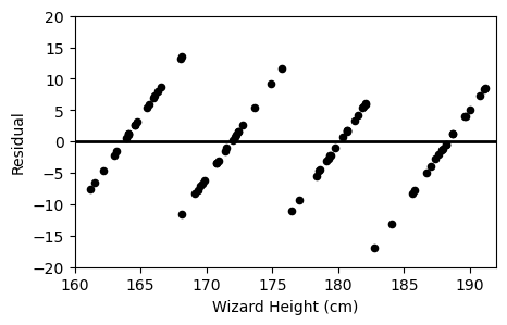
Which of the following plots is the residual plot for Professor Flitwick’s data?
Option A:
Option B:
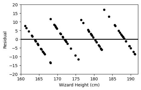
Option C:
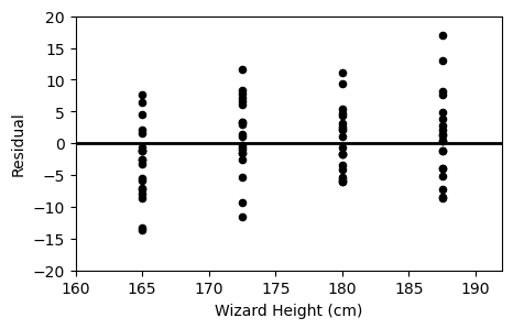
Answer: Option B
A residual plot shows the difference between actual and predicted values plotted against the predictor variable (x).
Since broomsticks come in specific sizes (150, 175, 200, 225 cm), the residuals will form slanted lines across the x axis.
We can immediately rule out Option C, as all the points lie on 4 specific wizard heights, which is totally different from the original plot.
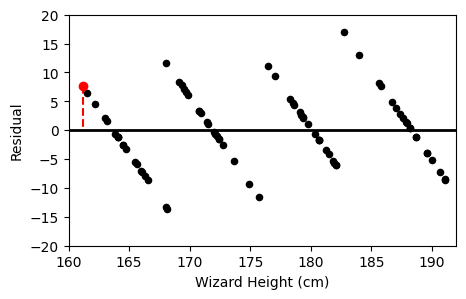
Now, if we were to pick a point:
 ,
,
We see that this point is above the line, meaning the difference between actual and predicted is positive (actual - predicted > 0)
Thus, if we were to check the point on option A or B, we see that option B’s graph corresponds with the original.
Option A

Option B
 ,
,
The average score on this problem was 59%.