← return to practice.dsc10.com
Below are practice problems tagged for Lecture 6 (rendered directly from the original exam/quiz sources).
Which type of visualization should we use to visualize the
distribution of "Range"?
Bar chart
Histogram
Scatter plot
Line plot
Answer: Histogram
"Range" is a numerical (i.e. quantitative) variable, and
we use histograms to visualize the distribution of numerical
variables.
"Range" is not
categorical."Range").
The average score on this problem was 63%.
Teslas, on average, tend to have higher "Range"s than
BMWs. In which of the following visualizations would we be able to see
this pattern? Select all that apply.
A bar chart that shows the distribution of "Brand"
A bar chart that shows the average "Range" for each
"Brand"
An overlaid histogram showing the distribution of
"Range" for each "Brand"
A scatter plot with "TopSpeed" on the x-axis and "Range" on the y-axis
Answer:
"Range" for each
"Brand""Range" for each "Brand"Let’s look at each option more closely.
Option 1: A bar chart showing the distribution
of "Brand" would only show us how many cars of each
"Brand" there are. It would not tell us anything about the
average "Range" of each "Brand".
Option 2: A bar chart showing the average range
for each "Brand" would help us directly visualize how the
average range of each "Brand" compares to one
another.
Option 3: An overlaid histogram, although
perhaps a bit messy, would also give us a general idea of the average
range of each "Brand" by giving us the distribution of the
"Range" of each brand. In the scenario mentioned in the
question, we’d expect to see that the Tesla distribution is further
right than the BMW distribution.
Option 4: A scatter plot of
"TopSpeed" against "Range" would only
illustrate the relationship between "TopSpeed" and
"Range", but would contain no information about the
"Brand" of each EV.
The average score on this problem was 91%.
Gabriel thinks "Seats" is a categorical variable because
it can be used to categorize EVs by size. For instance, EVs with 4 seats
are small, EVs with 5 seats are medium, and EVs with 6 or more seats are
large.
Is Gabriel correct?
Yes
No
Justify your answer in one sentence. Your answer must fit in the box below.
Answer: No
"Seats" is a numerical variable, since it makes sense to
do arithmetic with the values. For instance, we can find the average
number of "Seats" that a group of cars has. Gabriel’s
argument could apply to any numerical variable; just because we can
place numerical variables into “bins” doesn’t make them categorical.
The average score on this problem was 51%.
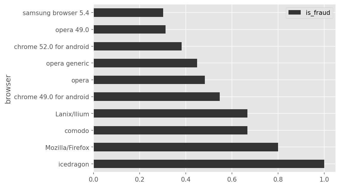
The following code block produces a bar chart, which is shown directly beneath it.
    (txn.groupby("browser").mean()
        .sort_values(by="is_fraud", ascending=False)
        .take(np.arange(10))
.plot(kind="barh", y="is_fraud"))Based on the above bar chart, what can we conclude about the browser
"icedragon"? Select all that apply.
In our dataset, "icedragon" is the most frequently used
browser among all transactions.
In our dataset, "icedragon" is the most frequently used
browser among fraudulent transactions.
In our dataset, every transaction made with "icedragon"
is fraudulent.
In our dataset, there are more fraudulent transactions made with
"icedragon" than with any other browser.
None of the above.
Answer: C
First, let’s take a look at what the code is doing. We start by
grouping by browser and taking the mean, so each column will have the
average value of that column for each browser (where each browser is a
row). We then sort in descending order by the "is_fraud"
column, so the browser which has the highest proportion of fraudulent
transactions will be first, and we take first the ten browsers, or those
with the most fraud. Finally, we plot the "is_fraud" column
in a horizontal bar chart. So, our plot shows the proportion of
fraudulent transactions for each browser, and we see that
icedragon has a proportion of 1.0, implying that every
transaction is fraudulent. This makes the third option correct. Since we
don’t have enough information to conclude any of the other options, the
third option is the only correct one.
The average score on this problem was 83%.
How can we modify the provided code block so that the bar chart displays the same information, but with the bars sorted in the opposite order (i.e. with the longest bar at the top)?
Change ascending=False to
ascending=True.
Add .sort_values(by="is_fraud", ascending=True)
immediately before .take(np.arange(10)).
Add .sort_values(by="is_fraud", ascending=True)
immediately after .take(np.arange(10)).
None of the above.
Answer: C
Let’s analyze each option A: This isn’t correct, because we must
remember that np.take(np.arange(10)) takes the rows indexed
0 through 10. And if we change ascending = False to
ascending = True, the rows indexed 0 through 10 won’t be
the same in the resulting DataFrame (since now they’ll be the 10
browsers with the lowest fraud rate). B: This will have
the same effect as option A, since it’s being applied before the
np.take() operation C: Once we have the 10 rows with the
highest fraud rate, we can sort them in ascending order in order to
reverse the order of the bars. Since we already have the 10 rows from
the original plot, this option is correct.
The average score on this problem was 59%.
You’re interested in comparing the "avg_housing_cost"
across different "family_type" groups for San Diego County,
CA specifically. Which type of visualization would be most
appropriate?
Scatter plot
Line plot
Bar chart
Histogram
Answer: Bar chart
"family_type" is a categorical variable, and we use bar
charts to visualize the distribution of categorical variables.
"avg_housing_cost")."family_type".
The average score on this problem was 89%.
Suppose we run the three lines of code below.
families = living_cost.groupby("family_type").median()
sorted_families = families.sort_values(by="avg_housing_cost")
result = sorted_families.get("avg_childcare_cost").iloc[0]
Which of the following does result evaluate to?
The median "avg_childcare_cost" of the
"family_type" with the lowest median
"avg_housing_cost".
The median "avg_childcare_cost" of the
"family_type" with the highest median
"avg_housing_cost".
The median "avg_housing_cost" of the
"family_type" with the lowest median
"avg_childcare_cost".
The median "avg_housing_cost" of the
"family_type" with the highest median
"avg_childcare_cost".
Answer: The median "avg_childcare_cost"
of the "family_type" with the lowest median
"avg_housing_cost".
When we grouped living_cost by
"family_type", families is a DataFrame with
one row per "family_type". Using the .median()
aggregation method takes the median of all numerical columns per
"family_type".
sorted_families is the families DataFrame,
but sorted in ascending order based on the
"avg_housing_cost" column. The first row of
sorted_families is the "family_type" with the
lowest median "avg_housing_cost", and the last row of
sorted_families is the "family_type" with the
highest median "avg_housing_cost".
In the last line of code, we’re getting the
"avg_childcare_cost" column from the
sorted_families DataFrame. We then use iloc to
get the first entry in the "avg_childcare_cost" column.
Since sorted_families is sorted in ascending order, this
means that we’re getting the lowest median in the column. Therefore,
result evaluates to the median
"avg_childcare_cost" of the "family_type" with
the lowest median "avg_housing_cost".
The average score on this problem was 82%.
Suppose we define another_result as follows.
another_result = (living_cost.groupby("state").count()
                  .sort_values(by="median_income", ascending=False)
                  .get("median_income").index[0])
What does another_result represent?
The state with the highest median income.
The median income in the state with the highest median income.
The state with the most counties.
The median income in the state with the most counties.
Answer: The state with the most counties.
The living_cost DataFrame is being grouped by the
"state" column, so there is now one row per
"state". By using the .count() aggregation
method, the columns in the DataFrame will contain the number of rows
in living_count for each "state". All of the
columns will also be the same after using .count(), so they
will all contain the distribution of "state". Since
living_cost has data on every county in the US, the grouped
DataFrame represents the number of counties that each state has.
We then sort the DataFrame in descending order, so the state with the
most counties is at the top of the DataFrame. The last line of the
expression gets a column and uses .index to get the state
corresponding to the first entry, which happens to be the state with the
most counties and the value that gets assigned to
another_result.
Since all the columns are the same, it doesn’t matter which column we
pick to use in the .sort_values() method. In this case, we
used the "median_income" column, but picking any other
column will produce the same result.
The average score on this problem was 65%.
Which of the following DataFrames has exactly four columns?
living_cost.groupby("family_type").min()
living_cost.groupby("family_type").sum()
living_cost.groupby("family_type").count()
None of the above.
Answer:
living_cost.groupby("family_type").sum()
Since we can’t take the sum of columns with categorical data, all of
the columns in living_cost that contain non-numerical data
are dropped after we use the .sum() aggregation method.
There are four columns in living_cost that have numerical
data ("is_metro", "avg_housing_cost",
"avg_childcare_cost", and "median_income").
Since Python can take the sum of these numerical columns, these four
columns are kept. Therefore, the resulting DataFrame has exactly four
columns.
Although "is_metro" contains Boolean values, Python can
still calculate the sum of this column. The Boolean value
True corresponds to 1 and False corresponds to
0.
The average score on this problem was 35%.
Suppose we define the Series three_columns to be the
concatenation of three columns of the living_cost DataFrame
as follows.
three_columns = (living_cost.get("state") + " " +
                 living_cost.get("county") + " " +
                 living_cost.get("family_type"))
For example, the first element of three_columns is the
string "CA San Diego County 1a2c" (refer back to the first
row of living_cost provided in the data overview).
What does the following expression evaluate to?
(living_cost.assign(geo_family=three_columns)
            .groupby("geo_family").count()
.shape[0]) 10, the number of distinct
"family_type" values.
50, the number of states in the US.
500, the number of combinations of
states in the US and "family_type" values.
3143, the number of counties in the US.
31430, the number of rows in the
living_cost DataFrame.
Answer: 31430, the
number of rows in the living_cost DataFrame.
The first line of the expression creates a new column in
living_cost, called "geo_family" that
represents the concatenation of the values in
"three_columns". When we group the DataFrame by
"geo_family", we create a new DataFrame that contains a row
for every unique value in "three_columns".
"three_columns" has various combinations of
"state", "country", and
"family_type". Since it’s given in the DataFrame
description that each of the 31430 rows of the DataFrame represents a
different combination of "state", "country",
and "family_type", this means that the grouped DataFrame
has 31430 unique combinations as well. Therefore, when we use
.shape[0] to get the number of rows in the grouped
DataFrame in the last line of the expression, we get the same value as
the number of rows in the living_cost DataFrame, 31430.
The average score on this problem was 74%.
Which type of plot should we use to visualize the distribution of the
"Location" column in the items DataFrame?
Scatter plot
Line plot
Bar chart
Histogram
Answer: Bar chart
The average score on this problem was 74%.
Notice that bookstore has an index of
"ISBN" and sales does not. Why is that?
There is no good reason. We could have set the index of
sales to "ISBN".
There can be two different books with the same
"ISBN".
"ISBN" is already being used as the index of
bookstore, so it shouldn’t also be used as the index of
sales.
The bookstore can sell multiple copies of the same book.
Answer: The bookstore can sell multiple copies of the same book.
In the sales DataFrame, each row represents an
individual sale, meaning multiple rows can have the same
"ISBN" if multiple copies of the same book are sold.
Therefore we can’t use it as the index because it is not a unique
identifier for rows of sales.
The average score on this problem was 87%.
Is "ISBN" a numerical or categorical variable?
numerical
categorical
Answer: categorical
Even though "ISBN" consists of numbers, it is used to
identify and categorize books rather than to quantify or measure
anything, thus it is categorical. It doesn’t make sense to compare ISBN
numbers like you would compare numbers on a number line, or to do
arithmetic with ISBN numbers.
The average score on this problem was 75%.
Which type of data visualization should be used to compare authors by median rating?
scatter plot
line plot
bar chart
histogram
Answer: bar chart
A bar chart is best, as it visualizes numerical values (median ratings) across discrete categories (authors).
The average score on this problem was 88%.
What would be the best type of plot to visualize the distribution of
"neighborhood" among the houses represented in
treat?
scatter plot
line plot
bar chart
histogram
Answer: bar chart
The average score on this problem was 76%.
Suppose we had access to historical data about the price of fun-sized candies over time. If we wanted to compare the prices of Milky Way and Skittles over time, which would be the best type of visualization to plot?
overlaid scatter plot
overlaid line plot
overlaid bar chart
overlaid histogram
Answer: overlaid line plot
The average score on this problem was 90%.
Below is a bar chart and the code that produced it.
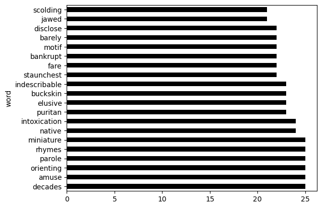
(words.sort_values(by="diff", ascending=False).take(np.arange(20))
      .plot(kind='barh', y="diff"));
Determine whether each statement below is true or false.
Students found the word “decades" more difficult than any other word.
True
False
Answer: False
We can see on the bar chart that there were 5 other words with the same diff value as decades, so the answer is False.
The average score on this problem was 83%.
If we removed ascending = False from the code, the bar
chart would show the same information, except the bars would appear in
the opposite order from top to bottom.
True
False
Answer: False
We are only plotting the first 20 rows of words after sorting it. So, currently we have plotted the 20 words with the highest diff value. If we removed ascending = False then it would sort in ascending order and we would only be plotting the 20 words with the lowest diff value. They would not be the same words.
The average score on this problem was 46%.
This bar chart shows all words that more than 20 students found
difficult. If we changed np.arange(20) to
np.arange(15) in the code, the bar chart would instead show
all words that more than 15 students found difficult.
True
False
Answer: False
.take(np.arange(20)) takes the elements at those
positional indices. .take(np.arange(15)) would take less
elements, so there is no way that it would include more students in the
bar chart
The average score on this problem was 80%.
Use the scatterplot of all 30 ingredients to determine how many have a calorie-to-protein ratio that is at least 5.
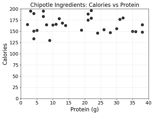
Answer: 26
The average score on this problem was 73%.
Let calories and protein be
numpy arrays containing the calorie and protein amounts, as
ints, for each of the 30 ingredients in chipotle. Fill in
the blanks so that the code below calculates the number of ingredients
with a calorie-to-protein ratio of at least 5.
count = __(a)__
for i in np.arange(__(b)__):
    if calories[i] / protein[i] >= 5:
count = __(c)__(a): 0
(b): len(calories)
(c): count + 1
The average score on this problem was 76%.
The expression below evaluates to True.
(
classify_artist('Michelle Branch')=='outdated'
and
classify_artist('Drake')=='trending'
)
Consider the scatterplot created by the code below.
merged.plot(kind='scatter', x='Year', y='Top_Hit_Year');The point for Drake is somewhere in this scatterplot. Relative to the point for Drake, there are four quadrants of the scatterplot, as shown below.
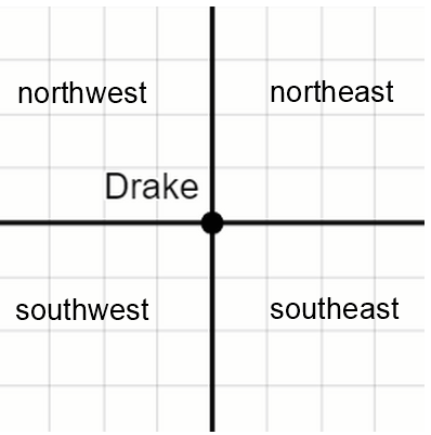
There is one quadrant in which the point for Michelle Branch cannot appear. Which is it?
northeast
northwest
southwest
southeast
Answer: northwest
The scatterplot shows an artist’s year of performance at Sun God on the x-axis, and their top hit year on the y-axis.
Since Drake is considered trending, we know his top hit came out within the five years prior to his Sun God performance. In other words, the time gap between his top hit release and his Sun God performance is at most five years.
If Michelle Branch were in the northwest quadrant, that would mean her x-coordinate was smaller than Drake’s, and her y-coordinate was larger. In other words, that would mean she performed at Sun God before Drake and her top hit was released after Drake’s. This means the time gap between her top hit release and her Sun God performance is less than five years, so she could not be considered outdated.
We could also answer this question through process of elimination. This would entail finding scenarios that show each of the other three quadrants is possible.
Michelle Branch could wind up in the northeast quadrant if, say, she performed 10 years after Drake and released her top hit 1 year after Drake. She’d be considered outdated because the time gap between her top hit and her Sun God performance would exceed five years.
Similarly, Michelle Branch could be in the southwest quadrant if, say, she performed 1 year before Drake and released her top hit 10 years before Drake. Again, the time gap between her top hit and her Sun God performance would exceed five years, making her outdated.
She could also be in the southeast quadrant if, say, she performed 10 years after Drake and released her top hit 10 years before Drake. This would also make the time gap between her top hit and Sun God performance more than five years.
So since all three other quadrants are possible and we are told that one quadrant is impossible, the northwest quadrant must be impossible.
The average score on this problem was 65%.
The scatter plot below shows the budget and revenue (in millions of
dollars) for each of the 6 distinct films in kate. Answer
each question below, or write “not enough info" if you don’t have enough
information to answer.
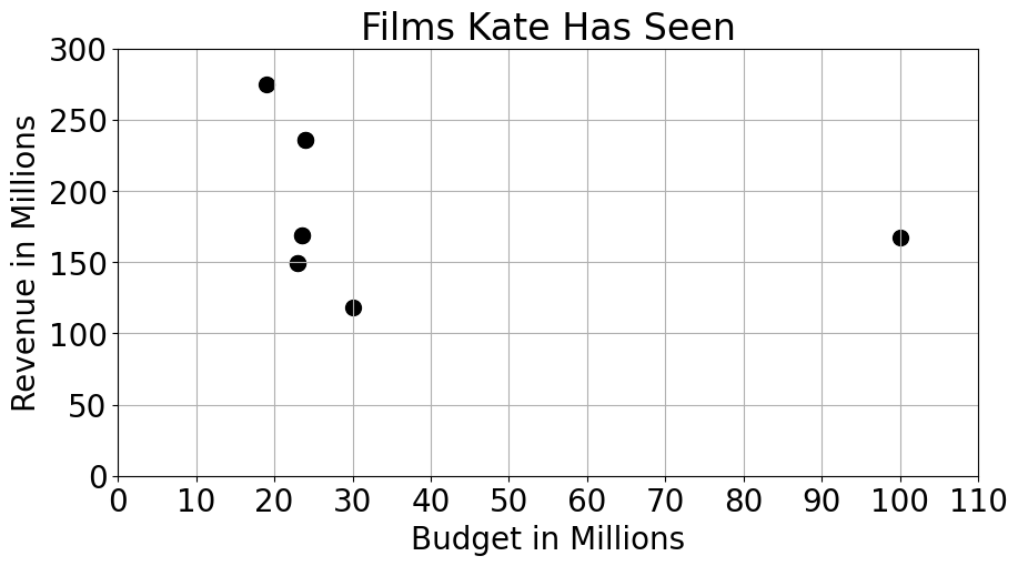
How many of these films had less than 200 million dollars in revenue?
Answer: 4
The average score on this problem was 98%.
How many of these films earned a revenue more than five times their budget?
Answer: 4
The average score on this problem was 85%.
Choose the best visualization to answer each of the following questions.
What kinds of dogs cost the most?
Bar plot
Scatter plot
Histogram
None
Answer: Bar plot
Here, there is a categorical variable (the breed of the dog) and a quantitative variable (the price of the dog). A bar plot is most suitable for this scenario when trying to compare quantitative values accross different categorical values. A scatter plot or histogram wouldn’t be appropriate here since both of those charts typically aim to visualize a comparison between two quantitative variables.
The average score on this problem was 89%.
Do toy dogs have smaller 'size' values than other
dogs?
Bar plot
Scatter plot
Histogram
None
Answer: None of the above
We are comparing two categorical variables ('size' and
'kind'). None of the graphs here are suitable for this
scenario since bar plots are used to compare a categorical variable
against a quantitative variable, while scatter plots and histograms
compare a quantitative variable against quantitative variable.
The average score on this problem was 26%.
Is there a linear relationship between weight and height?
Bar plot
Scatter plot
Histogram
None
Answer: Scatter plot
When looking for a relationship between two continuous quantitative variables, a scatter plot is the most appropriate graph here since the primary use of a scatter plot is to observe the relationship between two numerical variables. A bar chart isn’t suitable since we have two quantitative variables, while a bar chart visualizes a quantitative variable and a categorical variable. A histogram isn’t suitable since it’s typically used to show the frequency of each interval (in other words, the distribution of a numerical variable).
The average score on this problem was 100%.
Do dogs that are highly suitable for children weigh more?
Bar plot
Scatter plot
Histogram
None
Answer: Bar plot
We’re comparing a categorical variable (dog suitability for children) with a quantitative varible (weight). A bar plot is most approriate when comparing a categorical variable against a quantitative variable. Both scatter plot and histogram aim to compare a quantitative variable against another quantitative variable.
The average score on this problem was 40%.
Consider the scatterplot generated by the following expression:
kart.plot(kind="scatter, x="Total Points", y="Races Won")Which of the following questions would you be able to answer from this scatterplot? Select all that apply.
What is the name of the team that has the highest number of races won?
How many teams scored more than 6000 total points?
How many teams scored less than 100 total points per race that they won?
Which Division 2 school scored the most total points?
Answer:: Option 2 and Option 3
The average score on this problem was 95%.
We’d like to visualize the distribution of the "Mfr"
column in the laptops DataFrame. Fill in the blanks so that
the code below draws an appropriate plot.
laptops.groupby(__(a)__).__(b)__.get([__(c)__]).plot(kind=__(d)__)Answer:
Answer (a): "Mfr"
The average score on this problem was 92%.
Answer (b): count()
The average score on this problem was 82%.
Answer (c): "Model", "OS",
"Screen Size", or "Price"
The average score on this problem was 56%.
Answer (d): "bar" or
"barh"
The average score on this problem was 68%.
One of the clubs in the clubs DataFrame is the
"Surf Club". Without querying, write an
expression that evaluates to the rating of this club.
Answer:
clubs.set_index("Name").get("Rating").loc["Surf Club"]
The average score on this problem was 62%.
Now, using a query, write an expression that evaluates to the rating
of the "Surf Club".
Answer:
clubs[clubs.get("Name") == "Surf Club"].get("Rating").iloc[0]
The average score on this problem was 48%.
Fill in the blanks so the expression below evaluates to the name of
the category (e.g. "Social") with the largest number of
members, on average.
(clubs.groupby(__(a)__).__(b)__.sort_values(by="Members", ascending=__(c)__).__(d)__)Answer:
(a): "Category"
(b): mean()
(c): False
(d): index[0]
The average score on this problem was 59%.
In each category, what is the largest budget for a club? Write one line of code that would produce an appropriate data visualization to answer this question.
Answer:
clubs.groupby("Category").max().plot(kind= "bar", y= "Budget")
The average score on this problem was 38%.
For a report to the Academic Senate, you need to analyze course enrollment patterns. Write or finish one line of Python code that produces each quantity described.
(a) A DataFrame consisting of
"Department" as the index, and a single
column containing the mean "Enrollment" of all
courses within each "Department".
courses.get(["Department", "Enrollment"]).___________________________Answer: groupby("Department").mean() —
full one-liner:
courses.get(["Department", "Enrollment"]).groupby("Department").mean()
Explanation: .get(["Department", "Enrollment"]) keeps
only those columns. .groupby("Department") groups rows by
department. .mean() computes the mean of numeric columns
per group — here mean "Enrollment" — producing a DataFrame
with "Department" as the index and one column of means.
The average score on this problem was 78%.
(b) A scatter plot of the data in the
courses DataFrame with "Capacity" on the
x-axis and "Enrollment" on the y-axis.
Answer:
courses.plot(kind="scatter", x="Capacity", y="Enrollment")
kind="scatter" draws a scatter plot; x and
y name the columns for the horizontal and vertical
axes.
The average score on this problem was 79%.