← return to practice.dsc10.com
Below are practice problems tagged for Lecture 7 (rendered directly from the original exam/quiz sources).
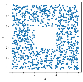
The seat-back TV on one of King Triton’s more recent flights was very
dirty and was full of fingerprints. The fingerprints made an interesting
pattern. We’ve stored the x and y positions of each fingerprint in the
DataFrame fingerprints, and created the following
scatterplot using
fingerprints.plot(kind='scatter', x='x', y='y')True or False: The histograms that result from the following two lines of code will look very similar.
fingerprints.plot(kind='hist',
                  y='x',
                  density=True,
                  bins=np.arange(0, 8, 2))
and
fingerprints.plot(kind='hist',
                  y='y',
                  density=True,
                  bins=np.arange(0, 8, 2))
True
False
Answer: True
The only difference between the two code snippets is the data values
used. The first creates a histogram of the x-values in
fingerprints, and the second creates a histogram of the
y-values in fingerprints.
Both histograms use the same bins:
bins=np.arange(0, 8, 2). This means the bin endpoints are
[0, 2, 4, 6], so there are three distinct bins: [0, 2), [2,
4), and [4, 6]. Remember the
right-most bin of a histogram includes both endpoints, whereas others
include the left endpoint only.
Let’s look at the x-values first. If we divide the
scatterplot into nine equally-sized regions, as shown below, note that
eight of the nine regions have a very similar number of data points.
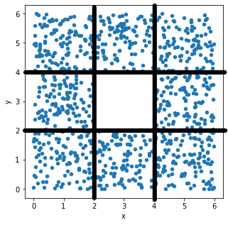
Aside from the middle region, about \frac{1}{8} of the data falls in each region.
That means \frac{3}{8} of the data has
an x-value in the first bin [0,
2), \frac{2}{8} of the data has
an x-value in the middle bin [2,
4), and \frac{3}{8} of the data
has an x-value in the rightmost bin [4, 6]. This distribution of
x-values into bins determines what the histogram will look
like.
Now, if we look at the y-values, we’ll find that \frac{3}{8} of the data has a
y-value in the first bin [0,
2), \frac{2}{8} of the data has
a y-value in the middle bin [2,
4), and \frac{3}{8} of the data
has a y-value in the last bin [4,
6]. That’s the same distribution of data into bins as the
x-values had, so the histogram of y-values
will look just like the histogram of x-values.
Alternatively, an easy way to see this is to use the fact that the
scatterplot is symmetric over the line y=x, the line that makes a 45 degree angle
with the origin. In other words, interchanging the x and
y values doesn’t change the scatterplot noticeably, so the
x and y values have very similar
distributions, and their histograms will be very similar as a
result.
The average score on this problem was 88%.
Below, we’ve drawn a histogram using the line of code
fingerprints.plot(kind='hist',
                  y='x',
                  density=True,
                  bins=np.arange(0, 8, 2))
However, our Jupyter Notebook was corrupted, and so the resulting histogram doesn’t quite look right. While the height of the first bar is correct, the histogram doesn’t contain the second or third bars, and the y-axis is replaced with letters.
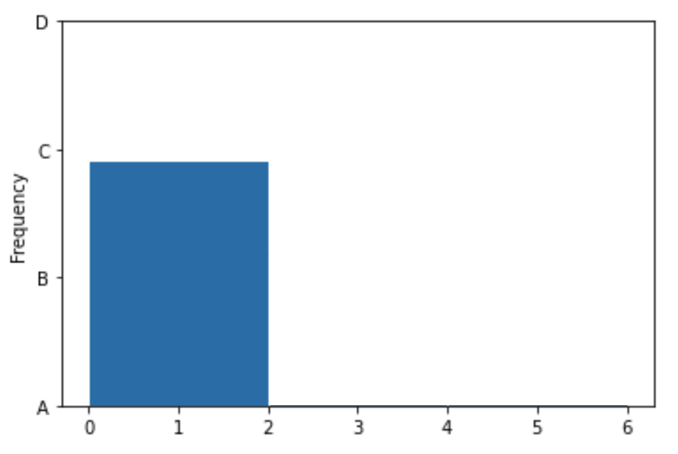
Which of the four options on the y-axis is closest to where the height of the middle bar should be?
A
B
C
D
Which of the four options on the y-axis is closest to where the height of the rightmost bar should be?
A
B
C
D
Answer: B, then C
We’ve already determined that the first bin should contain \frac{3}{8} of the values, the middle bin should contain \frac{2}{8} of the values, and the rightmost bin should contain \frac{3}{8} of the values. The middle bar of the histogram should therefore be two-thirds as tall as the first bin, and the rightmost bin should be equally as tall as the first bin. The only reasonable height for the middle bin is B, as it’s closest to two-thirds of the height of the first bar. Similarly, the rightmost bar must be at height C, as it’s the only one close to the height of the first bar.
The average score on this problem was 94%.
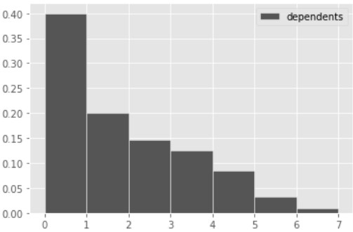
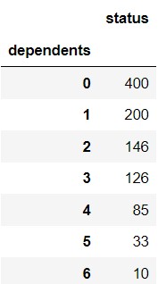
In this question, we’ll explore the number of dependents of each applicant. To begin, let’s define the variable dep_counts as follows.
dep_counts = apps.groupby("dependents").count().get(["status"])
The visualization below shows the distribution of the numbers of dependents per applicant. Note that every applicant has 6 or fewer dependents.
Use dep_counts and the visualization above to answer the
following questions.
What is the type of the variable dep_counts?
array
Series
DataFrame
Answer: DataFrame
As usual, .groupby produces a new DataFrame. Then we use
.get on this DataFrame with a list as the input, which
produces a DataFrame with just one column. Remember that
.get("status") produces a Series, but
.get(["status"]) produces a DataFrame
The average score on this problem was 78%.
What type of data visualization is shown above?
line plot
scatter plot
bar chart
histogram
Answer: histogram
This is a histogram because the number of dependents per applicant is a numerical variable. It makes sense, for example, to subtract the number of dependents for two applicants to see how many more dependents one applicant has than the other. Histograms show distributions of numerical variables.
The average score on this problem was 91%.
How many of the 1,000 applicants in apps have 2 or more
dependents? Give your answer as an integer.
Answer: 400
The bars of a density histogram have a combined total area of 1, and the area in any bar represents the proportion of values that fall in that bin.
In tihs problem, we want the total area of the bins corresponding to 2 or more dependents. Since this involves 5 bins, whose exact heights are unclear, we will instead calculate the proportion of all applicants with 0 or 1 dependents, and then subtract this proportion from 1.
Since the width of each bin is 1, we have for each bin, \begin{align*} \text{Area} &= \text{Height} \cdot \text{Width}\\ \text{Area} &= \text{Height}. \end{align*}
Since the height of the first bar is 0.4, this means a proportion of 0.4 applicants have 0 dependents. Similarly, since the height of the second bar is 0.2, a proportion of 0.2 applicants have 1 dependent. This means 1-(0.4+0.2) = 0.4 proportion of applicants have 2 or more dependents. Since there are 1,000 applicants total, this is 400 applicants.
The average score on this problem was 82%.
Define the DataFrame dependents_status as follows.
dependents_status = apps.groupby(["dependents", "status"]).count()
What is the maximum number of rows that
dependents_status could have? Give your answer as an
integer.
Answer: 14
When we group by multiple columns, the resulting DataFrame has one
row for each combination of values in those columns. Since there are 7
possible values for "dependents" (0, 1, 2, 3, 4, 5, 6) and
2 possible values for "status" ("approved",
"denied"), this means there are 7\cdot 2 = 14 possible combinations of values
for these two columns.
The average score on this problem was 59%.
Recall that dep_counts is defined as follows.
dep_counts = apps.groupby("dependents").count().get(["status"])
Below, we define several more variables.
variable1 = dep_counts[dep_counts.get("status") >= 2].sum()

variable2 = dep_counts[dep_counts.index > 2].get("status").sum()

variable3 = (dep_counts.get("status").sum()
            - dep_counts[dep_counts.index < 2].get("status").sum())

variable4 = dep_counts.take(np.arange(2, 7)).get("status").sum()

variable5 = (dep_counts.get("status").sum()
            - dep_counts.get("status").loc[1]
            - dep_counts.get("status").loc[2])
Which of these variables are equal to your answer from part (c)? Select all that apply.
variable1
variable2
variable3
variable4
variable5
None of the above.
Answer: variable3,
variable4
First, the DataFrame dep_counts is indexed by
"dependents" and has just one column, called
"status" containing the number of applicants with each
number of dependents. For example, dep_counts may look like
the DataFrame shown below.
variable1 does not work because it doesn’t make sense to
query with the condition dep_counts.get("status") >= 2.
In the example dep_counts shown above, all rows would
satisfy this condition, but not all rows correspond to applicants with 2
or more dependents. We should be querying based on the values in the
index instead.
variable2 is close but it uses a strict inequality
> where it should use >= because we want
to include applicants with 2 dependents.
variable3 is correct. It uses the same approach we used
in part (c). That is, in order to calculate the number of applicants
with 2 or more dependents, we calculate the total number of applicants
minus the number of applicants with less than 2 dependents.
variable4 works as well. The strategy here is to keep
only the rows that correspond to 2 or more dependents. Recall that
np.arange(2, 7) evaluates to the array
np.array([2, 3, 4, 5, 6]). Since we are told that each
applicant has 6 or fewer dependents, keeping only these rows
correspondings to keeping all applicants with 2 or more dependents.
variable5 does not work because it subtracts away the
applicants with 1 or 2 dependents, leaving the applicants with 0, 3, 4,
5, or 6 dependents. This is not what we want.
The average score on this problem was 77%.
Next, we define variables x and y as
follows.
x = dep_counts.index.values
y = dep_counts.get("status")Note: If idx is the index of a Series or
DataFrame, idx.values gives the values in idx
as an array.
Which of the following expressions evaluate to the mean number of dependents? Select all that apply.
np.mean(x * y)
x.sum() / y.sum()
(x * y / y.sum()).sum()
np.mean(x)
(x * y).sum() / y.sum()
None of the above.
Answer: (x * y / y.sum()).sum(),
(x * y).sum() / y.sum()
We know that x is
np.array([0, 1, 2, 3, 4, 5, 6]) and y is a
Series containing the number of applicants with each number of
dependents. We don’t know the exact values of the data in
y, but we do know there are 7 elements that sum to 1000,
the first two of which are 400 and 200.
np.mean(x * y) does not work because x * y
has 7 elements, so np.mean(x * y) is equivalent to
sum(x * y) / 7, but the mean number of dependents should be
sum(x * y) / 1000 since there are 1000 applicants.
x.sum() / y.sum() evaluates to \frac{21}{1000} regardless of how many
applicants have each number of dependents, so it must be incorrect.
(x * y / y.sum()).sum() works. We can think of
y / y.sum() as a Series containing the proportion of
applicants with each number of dependents. For example, the first two
entries of y / y.sum() are 0.4 and 0.2. When we multiply
this Series by x and sum up all 7 entries, the result is a
weighted average of the different number of dependents, where the
weights are given by the proportion of applicants with each number of
dependents.
np.mean(x) evaluates to 3 regardless of how many
applicants have each number of dependents, so it must be incorrect.
(x * y).sum() / y.sum() works because the numerator
(x * y).sum() represents the total number of dependents
across all 1,000 applicants and the denominator is the number of
applicants, or 1,000. The total divided by the count gives the mean
number of dependents.
The average score on this problem was 71%.
What does the expression y.iloc[0] / y.sum() evaluate
to? Give your answer as a fully simplified
fraction.
Answer: 0.4
y.iloc[0] represents the number of applicants with 0
dependents, which is 400. y.sum() represents the total
number of applicants, which is 1,000. So the ratio of these is 0.4.
The average score on this problem was 73%.
Histograms A and B below both display the distribution of the
"Seats" column, using different bins. Each histogram
includes all 32 rows of evs.
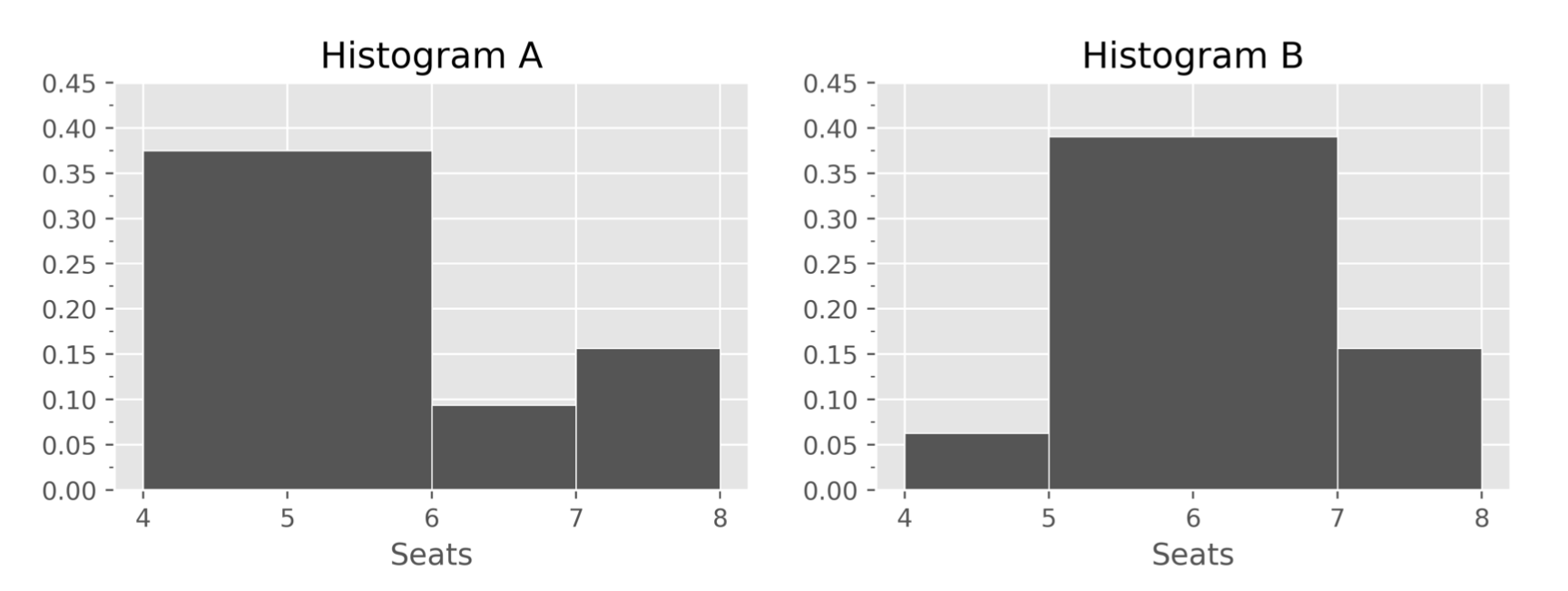
How many EVs in evs have exactly 6 seats?
Answer: 3
Here are two ways to solve this problem. In both solutions, we only
look at Histogram A, since only Histogram A contains a bin that
corresponds to EVs with exactly 6 "Seats". Recall, in
histograms, bins are inclusive of the left endpoint and exclusive of the
right endpoint, which means the [6, 7) bin represents EVs with >= 6
"Seats" and < 7 "Seats"; since the number
of "Seats" is a whole number, this corresponds to exactly 6
"Seats".
Solution 1
Since the bin [6, 7) has a width of 1, its height is equal to its area, which is equal to the proportion of values in that bin. There are 32 values total, so all proportions (and, thus, the height of the [6, 7) bar) must be a multiple of \frac{1}{32}. The height is close to but just under 0.01; this implies the height is \frac{3}{32}, since that is also close to but just under 0.01 (\frac{4}{32} is way above and \frac{2}{32} is way below). So, we conclude that the number of EVs with 6 seats is 3.
Solution 2
The height of the [6, 7) bar is ever-so-slightly less than 0.1. If it’s height was 0.1, it would imply that the proportion of values in the [6, 7) bin was 0.1 \cdot (7 - 6) = 0.1, which would imply that the number of values in the [6, 7) bin is 0.1 \cdot 32 = 3.2. However, since the number of values in a bin must be an integer, the number of values in this bin is 3 (which is slightly less than 3.2).
The average score on this problem was 61%.
How many EVs in evs have exactly 5 seats?
Answer: 22
Now, we must look at Histogram B. In the previous part, we computed
that there are 3 EVs with exactly 6 "Seats" in
evs. Histogram B shows us the proportion, and thus number,
of EVs with 5 or 6 "Seats", through its [5, 7) bin
(remember, this bin corresponds to EVs with >= 5 "Seats"
and < 7 "Seats"). If we can find the number of EVs with
5 or 6 "Seats", we can subtract 3 from it to determine the
number of EVs with exactly 5 "Seats".
Since it’s not quite clear what the height of the [5, 7) bar is, we can create a range for the height of the bar, and use that to come up with a range for the area of the bar, and hence a range for the number of values in the bin. We can then use the fact that the number of values in a bin must be an integer to narrow down our answer.
"Seats" is less than 0.8, and the number of EVs with 5 or
6 "Seats" is less than 0.8 \cdot
32 = 25.6."Seats" is more than 0.75 \cdot
32 = 24.We’ve found that the number of EVs with 5 or 6 "Seats"
is more than 24 and less than 25.6. There is only one integer in this
range – 25 – so the number of EVs with 5 or 6 "Seats" is
25. Finally, the number of EVs with exactly 5 seats is 25 - 3 = 22.
The average score on this problem was 35%.
Histogram C also displays the distribution of the
"Seats" column, but uses just a single bin, [4, 9]. What is
the height of the sole bar in Histogram C?
Answer: \frac{1}{5} (or 0.2)
Recall, the total area of a (density) histogram is 1. Since Histogram C only has one bar, the area of that one bar must be 1. we can use this fact to find what its height must be.
\begin{align*} \text{Area} &= \text{Width} \cdot \text{Height} \\ 1 &= (9 - 4) \cdot \text{Height} \\ \frac{1}{5} &= \text{Height} \end{align*}
The average score on this problem was 68%.
Ashley doesn’t have access to the entire txn DataFrame;
instead, she has access to a simple random sample of
400 rows of txn.
She draws two histograms, each of which depicts the distribution of
the "amount" column in her sample, using different
bins.
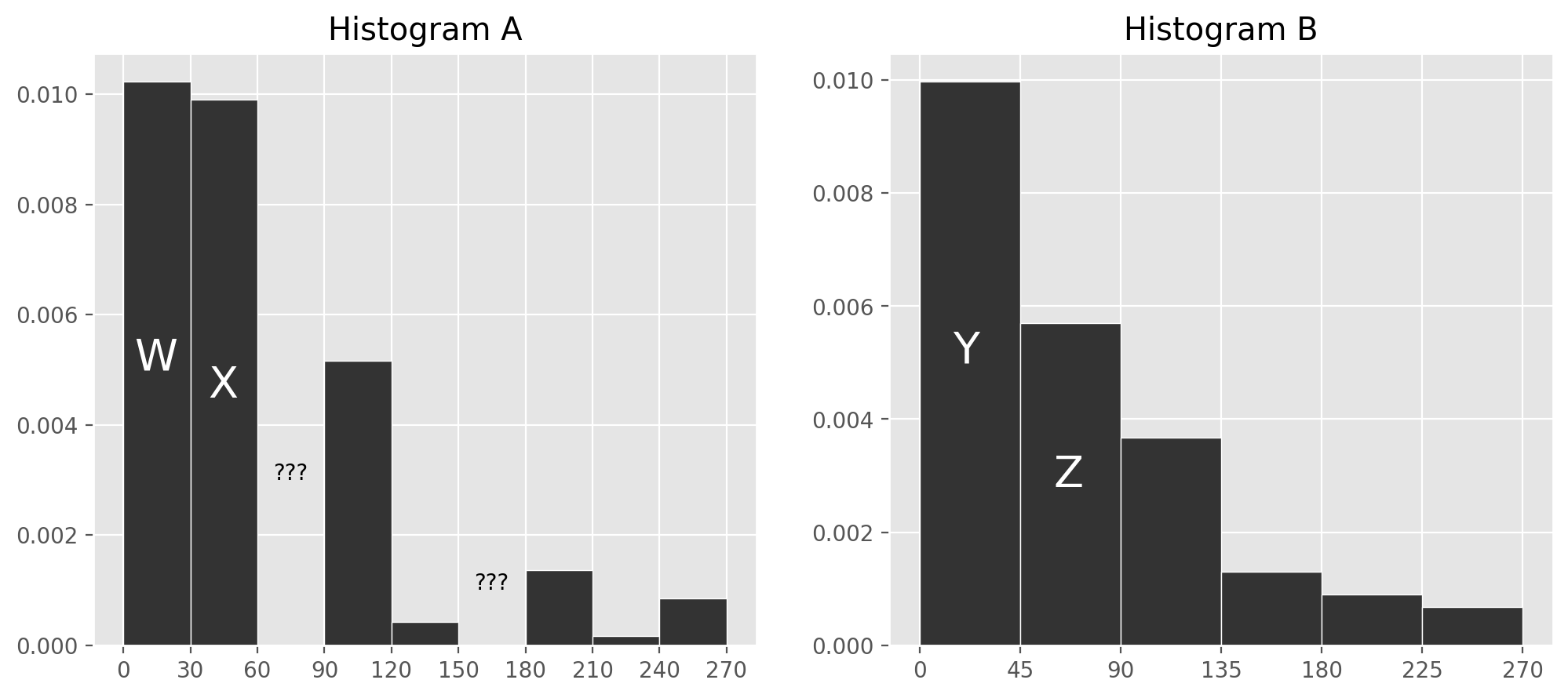
Unfortunately, DataHub is being finicky and so two of the bars in Histogram A are deleted after it is created.
In Histogram A, which of the following bins contains approximately 60 transactions?
[30, 60)
[90, 120)
[120, 150)
[180, 210)
Answer: [90, 120)
The number of transactions contained in the bin is given by the area of the bin times the total number of transactions, since the area of a bin represents the proportion of transactions that are contained in that bin. We are asked which bin contains about 60 transactions, or \frac{60}{400} = \frac{3}{20} = 0.15 proportion of the total area. All the bins in Histogram A have a width of 30, so for the area to be 0.15, we need the height h to satisfy h\cdot 30 = 0.15. This means h = \frac{0.15}{30} = 0.005. The bin [90, 120) is closest to this height.
The average score on this problem was 90%.
Let w, x, y, and z be the heights of bars W, X, Y, and Z, respectively. For instance, y is about 0.01.
Which of the following expressions gives the height of the bar corresponding to the [60, 90) bin in Histogram A?
( y + z ) - ( w + x )
( w + x ) - ( y + z )
\frac{3}{2}( y + z ) - ( w + x )
( y + z ) - \frac{3}{2}( w + x )
3( y + z ) - 2( w + x )
2( y + z ) - 3( w + x )
None of the above.
Answer: \frac{3}{2}( y + z ) - ( w + x )
The idea is that the first three bars in Histogram A represent the same set of transactions as the first three bars of Histogram B. Setting these areas equals gives 30w+30x+30u= 45y+45z, where u is the unknown height of the bar corresponding to the [60, 90) bin. Solving this equation for u gives the result.
\begin{align*} 30w+30x+30u &= 45y+45z \\ 30u &= 45y+45z-30w-30x \\ u &= \frac{45y + 45z - 30w - 30x}{30} \\ u &= \frac{3}{2}(y+z) - (w+x) \end{align*}
The average score on this problem was 50%.
The rows in living_cost with a
"family_type" value of "1a0c" correspond to
families that consist of individuals living on their own. We’ll call
such families “solo families." Below, we’ve visualized the distribution
of the "median_income" column, but only for rows
corresponding to solo families. Instead of visualizing median incomes in
dollars, we’ve visualized them in thousands of dollars.
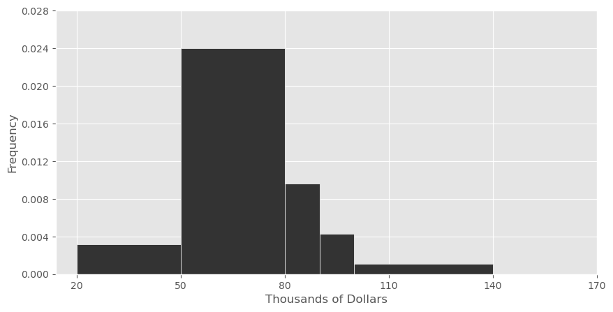
Suppose we’re interested in splitting the [50, 80) bin into two separate bins — a [50, 70) bin and a [70, 80) bin.
Let h_1 be the height of the new bar corresponding to the [50, 70) bin and let h_2 be the height of the new bar corresponding to the [70, 80) bin.
What are the minimum and maximum possible values of h_2? Give your answers as decimals rounded to three decimal places.
Answer: Minimum: 0
In a histogram, we do not know how data are distributed within a bin. This means that when we split the bin with range [50, 80) into two smaller bins, we have no way of knowing how the data from the original bin will be distributed. It is possible that all of the data in the [50, 80) bin fell between 50 and 70. In this case, there would be no data in the [70, 80) bin, and as such, the height of this new bar would be 0.
The average score on this problem was 61%.
Answer: Maximum: 0.072
Similarly, if all of the data in the original [50,80) bin fell between 70 and $80, then all of the data that was originally in the [50, 80) bin would be allocated to the [70, 80) bin. In a density histogram, the area of a bar corresponds to the proportion of the data contained within the bar (for example, a bar with area 0.5 contains 50% of the total data). Since the maximum value of h_2 is achieved when the bin [70, 80) contains all of the data originally contained in the bin [50, 80), this means area of the [70, 80) bar must be the same as the original area of the [50, 80) bar, since it contains the same proportion of data.
The original bar had area 30 * 0.024 = 0.72, which comes from multiplying its base and its height. Since the new bar has a base of 10, its height must be 0.072 to make its area equal to 0.72. Intuitively, if a rectangle is one third as wide as another rectangle and has the same area, it must be three times as tall.
The average score on this problem was 42%.
Suppose that the number of counties in which the median income of solo families is in the interval [50, 70) is r times the number of counties in which the median income of solo families is in the interval [70, 80). Given this fact, what is the value of \frac{h_1}{h_2}, the ratio of the heights of the two new bars?
\frac{1}{r}
\frac{2}{r}
\frac{3}{r}
\frac{r}{2}
\frac{r}{3}
2r
3r
Answer: \frac{r}{2}
The key to solving this problem is recognizing that the number of counties in a given interval is directly related to the area of that interval’s bar in the histogram. This comes from the property of density histograms that the area of a bar corresponds to the proportion of the data contained within the bar.
Given that there are r times the amount of data in the interval [50, 70), in comparison to the interval [70, 80), we know that the area of the bar corresponding to the bin [50, 70) is r times the area of the bar corresponding to the bin [70, 80).
Therefore, if A_1 represents the area of the [50, 70) bar and A_2 represents the area of the [70, 80) bar, we have
A_1 = r \cdot A_2.
Then, since each bar is a rectangle, its area comes from the product of its height and its base. We know the [50, 70) bar has a base of 20 and a height of h_1, and the [70, 80) bar has a base of 10 and a height of h_2. Plugging this in gives
h_1 \cdot 20 = r \cdot h_2 \cdot 10.
From here, we can rearrange terms to get
\frac{h_1}{h_2} = \frac{r}{2}.
The average score on this problem was 40%.
Nintendo collected data on the heights of a sample of Animal Crossing: New Horizons players. A histogram of the heights in their sample is given below.
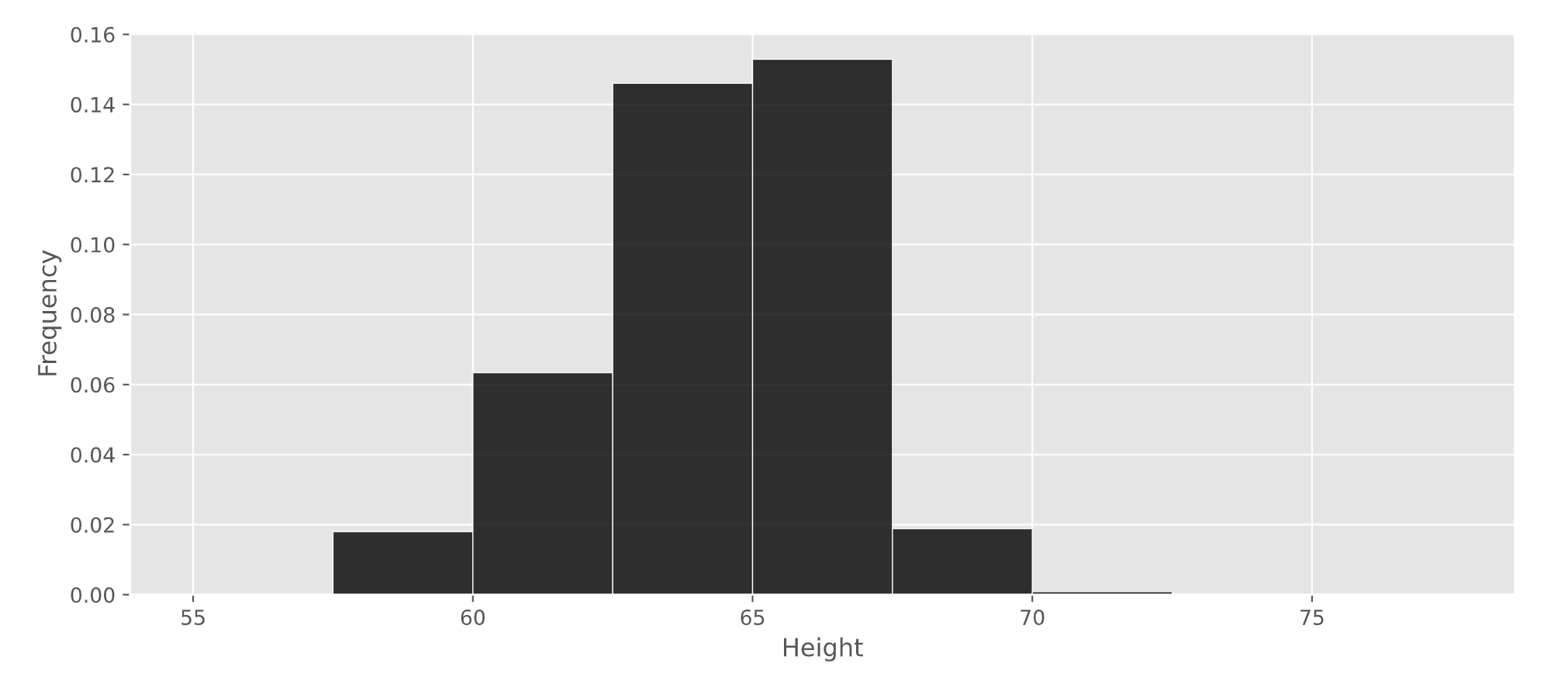
What percentage of players in Nintendo’s sample are at least 62.5 inches tall? Give your answer as an integer rounded to the nearest multiple of 5.
Answer: 80%
The average score on this problem was 73%.
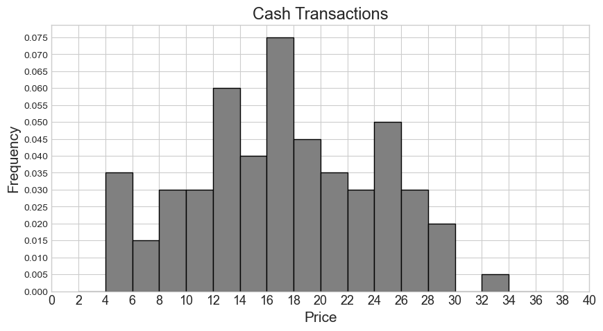
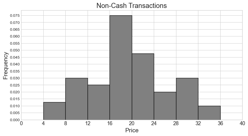
Suppose we are told that sales contains 1000 rows, 500
of which represent cash transactions and 500 of which represent non-cash
transactions. We are given two density histograms representing the
distribution of "price" separately for the cash and
non-cash transactions.
From these two histograms, we’d like to create a single combined
histogram that shows the overall distribution of "price"
for all 1000 rows in sales.
How many cash transactions had a "price" of \$26 or more?
Answer: 55
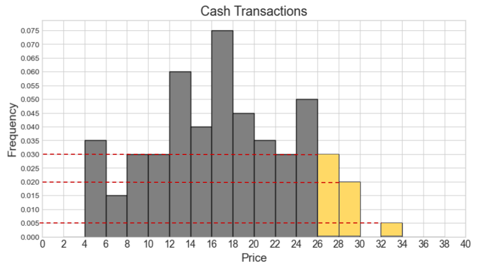
We first locate the bars representing \$26 or more on the cash transaction histogram, which are the three rightmost bars. We then calculate the area of these bars to get the proportion of cash transactions these bars correspond to.
\textit{Area} = 0.03 * 2 + 0.02 * 2 + 0.005 * 2 = 0.06 + 0.04 + 0.01 = 0.11
Lastly, we multiply this proportion by the total count of 500 to get
the count of transactions with a "price" of \$26 or more.
\text{number of transactions} = 0.11 * 500 = 55
The average score on this problem was 64%.
Say our combined histogram has a bin [4, 6). What will the height of this bar be in the combined histogram? Fill in the answer box or select “Not enough information.”
Answer: Not enough information.
Since the histogram for non-cash transactions only has a bin of [4, 8), we don’t have enough information about how many of these transactions fall within [4, 6). In general, we can’t tell where within a bin values fall in a histogram.
The average score on this problem was 81%.
Say our combined histogram has a bin [24, 28). What will the height of this bar be in the combined histogram? Fill in the answer box or select “Not enough information.”
Answer: 0.03
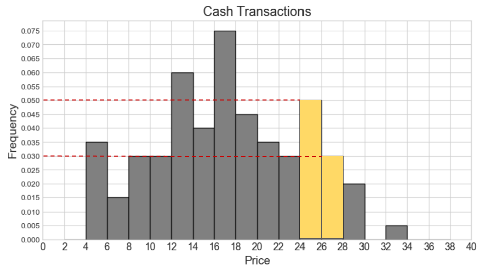
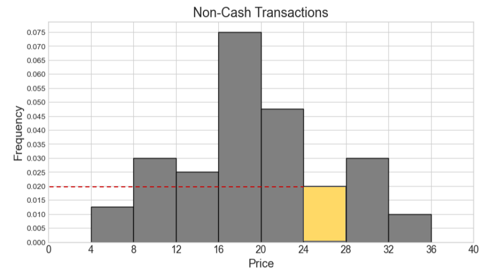
We first calculate the counts for cash and non-cash transactions within [24, 28) separately. Then we add the two counts and find the proportion this represents out of 1000 total transactions. Lastly, we determine the height of the bar by dividing the area (proportion) by the width 4.
Number of cash transactions within [24, 28) = (0.05 * 2 + 0.03 * 2) * 500 = (0.1 + 0.06) * 500 = 0.16 * 500 = 80
Number of non-cash transactions within [24, 28) = (0.02 * 4) * 500 = 0.08 * 500 = 40
Total number of transactions within [24, 28) = 80 + 40 = 120
Proportion of one thousand total transactions (area of bar) = 120 / 1000 = 0.12
Height of bar = 0.12 / 4 = 0.03
The average score on this problem was 42%.
Suppose now that the histograms for cash and non-cash transactions are the same as pictured, but they now represent 600 cash transactions and 400 non-cash transactions. In this situation, say our combined histogram has a bin [12, 16). What will the height of this bar be in the combined histogram? Fill in the answer box or select “Not enough information.”
Answer: 0.04
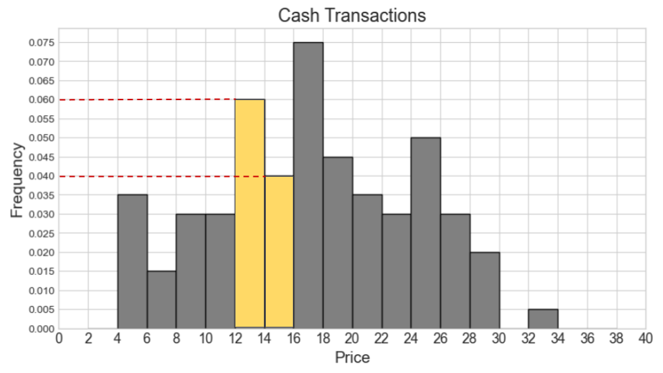
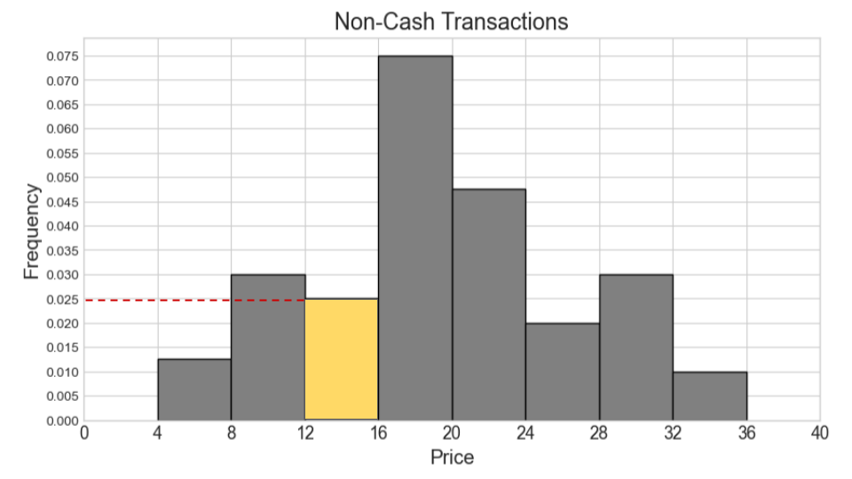
We can use the same process as we used for the previous part. We first calculate the counts for cash and non-cash transactions within [12, 16) separately. Then we add the two counts and find the proportion this represents out of 1000 total transactions. Lastly, we determine the height of the bar by dividing the area (proportion) by the width 4.
Number of cash transactions within [12, 16) = (0.06 * 2 + 0.04 * 2) * 600 = (0.12 + 0.08) * 600 = 0.2 * 600 = 120
Number of non-cash transactions within [12, 16) = (0.025 * 4) * 400 = 0.1 * 400 = 40
Total number of transactions within [12, 16) = 120 + 40 = 160
Proportion of one thousand total transactions (area of bar) = 160 / 1000 = 0.16
Height of bar = 0.16 / 4 = 0.04
The average score on this problem was 37%.
Recall from the last problem that the DataFrame
trick_or_treat includes a column called
"price" with the cost in dollars of a single
piece of fun-sized candy, as a float.
Assume we have run the line of code tot = trick_or_treat
to reassign trick_or_treat to the shorter variable name
tot.
In this problem, we’ll use tot to calculate the total
amount of money that each house spent on Halloween candy. This number is
always less than \$80 for the houses in
our data set.
Fill in the blanks below so that the following block of code plots a histogram that displays the distribution of the total amount of money that houses spent on Halloween candy, in dollars.
total = (tot.assign(total_spent = ___(a)___)
            .groupby(___(b)___).___(c)___)
total.plot(kind = "hist",  y = "total_spent", density = True,
           bins = np.arange(0, 90, 10))
Answer:
(a): tot.get("price") * tot.get("how_many")
(b): “address”
(c): sum()
(a):
tot.get("price") * tot.get("how_many")
tot.get("price") retrieves the cost of a single piece
of candy.tot.get("how_many") retrieves the number of pieces of
candy given out.total_spent that
represents the total money spent for each type of candy at a given
house.(b): “address”
"address" column, which
uniquely identifies each house. This ensures that all records associated
with a single house are aggregated together.(c): sum()
"address", the .sum()
operation aggregates the total amount of money spent on candy for each
house. This sums up all total_spent values for records
belonging to the same house.Final Output: The total DataFrame will have one row for
each house, with the column total_spent representing the
total money spent on Halloween candy. Finally, the
total.plot command creates a histogram of the
total_spent values to visualize the distribution of
spending across houses.
The average score on this problem was 65%.
The histogram below displays the distribution of the total amount of money that houses spent on Halloween candy; it is the histogram that would be generated from the code snippet above, assuming the blanks were filled in correctly.

Which two adjacent bins in the histogram represent about 50\% of the houses?
[10, 20) and [20, 30)
[20, 30) and [30, 40)
[30, 40) and [40, 50)
[40, 50) and [50, 60)
[50, 60) and [60, 70)
Not possible to determine.
Answer: [20, 30) and
[30, 40)
[20, 30) and
[30, 40) have the two tallest bars, with heights of 0.020
and 0.030, respectively.[20, 30) contributes 0.020
\times 10 = 0.2 or 20\% of the
houses.[30, 40) contributes 0.030
\times 10 = 0.3 or 30\% of the
houses.
The average score on this problem was 83%.
Suppose we create a new histogram, using the same code as above but
with bins = np.arange(0, 90, 20) instead of
bins = np.arange(0, 90, 10). Approximate the height of the
tallest bar in this new histogram. If this is not possible, write “Not
possible to determine."
Answer: 0.025
[0, 20),[20, 40),[40, 60),[60, 80).
The bin [20, 40) merges the original bins
[20, 30) and [30, 40) and would be the bin
with the highest bar in the new histogram.[20, 40):
[20, 30) contributes 0.020
\times 10 = 0.2 (20%).[30, 40) contributes 0.030
\times 10 = 0.3 (30%).[20, 40) is 0.2 +
0.3 = 0.5 or 50\%.
The average score on this problem was 38%.
Suppose we create a new histogram, using the same code as above but
substituting bins = np.arange(0, 90, 5) for
bins = np.arange(0, 90, 10). Approximate the height of the
tallest bar in this new histogram. If this is not possible, write “Not
possible to determine."
Answer: Not possible to determine.
[20, 30)). When switching to 5-unit bins (e.g.,
[20, 25), [25, 30)), we need to know the
distribution of data within the original 10-unit bins to calculate the
new bar heights.[20, 30)
is evenly distributed between [20, 25) and
[25, 30) or concentrated in one of the sub-bins.
The average score on this problem was 70%.
Suppose we plot a density histogram showing the distribution of the
"Degrees" column in uc, using the argument
bins=np.arange(0, uc.get("Degrees").max() + 3000, 2000)
.
Suppose there are 12 rows of uc corresponding to
campuses and years in which fewer than 2000 degrees were awarded. How
tall will the first bar in the histogram be? Give your answer as an
exact decimal or simplified fraction.
Answer: 0.0001
The average score on this problem was 33%.
The DataFrame long was created by taking the 500 rows of words corresponding
to words whose "length" is more than 10. Of the 500 words in long,
The density histogram below was created using the data in the
"diff" column of long. The bins
argument was set as bins=np.arange(5, 30, 5) so the
histogram does not include words that fewer than 5
students marked difficult.
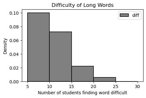
How many words were marked difficult by 10 or more students? Give your answer as an integer.
Answer: 50
To find the number of words marked difficult by 10 or more students,
we can calculate 100 \; - {the number
of words marked difficult by at least 5 students or less than 10
students}, or 100 \; - {the number of
words in bin [5,10)}.
Number of words in bin [5,10) =
(5)(.10)(100) = 50
100 - 50 = 50 words marked difficult
by at least 10 students.
We can also use 1 \; - {proportion of total words in bin [5,10)}, then multiply by 100. Similarly, we can directly calculate the necessary proportion of students by using the area of 3 rightmost bins.
Suppose we regenerated the histogram using the same data, but setting
the bins argument as
bins=np.arange(0, 30, 5).
What would be the height of the bar [5, 10)? Give your answer as a decimal number.
What would be the height of the bar [0, 5)? Give your answer as a decimal number.
Answer (Part 1): 0.02
We know that there are 50 words in the bin [5,10).
Now, however, the histogram is showing all 500 words. So the proportion
of words in bin [5,10) is \frac{50}{500} = 0.1.
To find the height of bar [5,10), we
use:
5 \cdot {h} = 0.1
h = \frac{0.1}{5} = 0.02
Answer (Part 2): 0.16
We know that 100 words were marked difficult by 5 or more students,
so that means 500 - 100 = 400 words
were marked difficult by less than 5 students.
So \frac{400}{500} = 0.8 =
{proportion of total words that less than 5 students found
difficult}.
To find the height of bar [0,5), we use:
5 \cdot {h} = 0.8
h = \frac{0.8}{5} = 0.16
The average score on this problem was 57%.
Below is a density histogram showing the distribution of calories for
all 30 ingredients in chipotle.
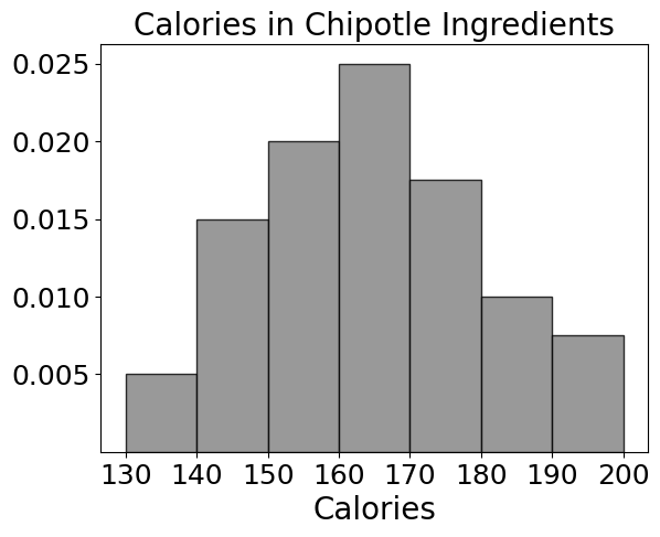
How many ingredients have less than 160 calories?
Answer: 12
The average score on this problem was 83%.
Suppose we had plotted the histogram with the argument
bins=[120, 160, 190, 210].
(i): 3
(ii): 0.01
The average score on this problem was 63%.
The histogram below shows the distribution of the number of products sold per day throughout the last 30 days, for two different IKEA products: the KURA reversible bed, and the ANTILOP highchair.
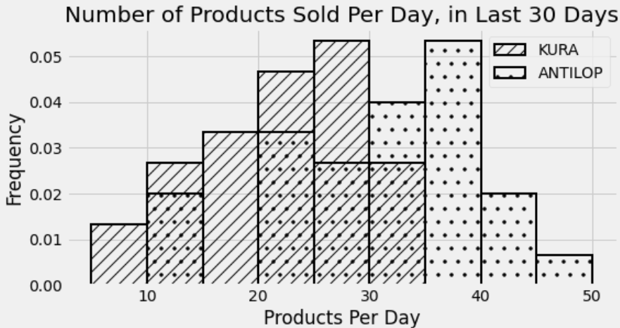
For how many days did IKEA sell between 20 (inclusive) and 30 (exclusive) KURA reversible beds per? Give an integer answer or write “not enough information”, but not both.
Answer: 15
Remember that for a density histogram, the proportion of data that falls in a certain range is the area of the histogram between those bounds. So to find the proportion of days for which IKEA sold between 20 and 30 KURA reversible beds, we need to find the total area of the bins [20, 25) and [25, 30). Note that the left endpoint of each bin is included and the right bin is not, which works perfectly with needing to include 20 and exclude 30.
The bin [20, 25) has a width of 5 and a height of about 0.047. The bin [25, 30) has a width of 5 and a height of about 0.053. The heights are approximate by eye, but it appears that the [20, 25) bin is below the horizontal line at 0.05 by the same amount which the [25, 30) is above that line. Noticing this spares us some annoying arithmetic and we can calculate the total area as
\begin{aligned} \text{total area} &= 5*0.047 + 5*0.053 \\ &= 5*(0.047 + 0.053) \\ &= 5*(0.1) \\ &= 0.5 \end{aligned}
Therefore, the proportion of days where IKEA sold between 20 and 30 KURA reversible beds is 0.5. Since there are 30 days represented in this histogram, that corresponds to 15 days.
The average score on this problem was 54%.
For how many days did IKEA sell more KURA reversible beds than ANTILOP highchairs? Give an integer answer or write “not enough information”, but not both.
Answer: not enough information
We cannot compare the number of KURA reversible beds sold on a certain day with the number of ANTILOP highchairs sold on the same day. These are two separate histograms shown on the same axes, but we have no way to associate data from one histogram with data from the other. For example, it’s possible that on some days, IKEA sold the same number of KURA reversible beds and ANTILOP highchairs. It’s also possible from this histogram that this never happened on any day.
The average score on this problem was 54%.
Determine the relative order of the three quantities below.
(1)<(2)<(3)
(1)<(3)<(2)
(2)<(1)<(3)
(2)<(3)<(1)
(3)<(1)<(2)
(3)<(2)<(1)
Answer: (2)<(3)<(1)
We can calculate the exact value of each of the quantities:
To find the number of days for which IKEA sold at least 35 ANTILOP highchairs, we need to find the total area of the rightmost three bins of the ANTILOP distribution. Doing a similar calculation to the one we did in Problem 11.1, \begin{aligned} \text{total area} &= 5*0.053 + 5*0.02 + 5*0.007 \\ &= 5*(0.08) \\ &= 0.4 \end{aligned} This is a proportion of 0.4 out of 30 days total, which corresponds to 12 days.
To find the number of days for which IKEA sold less than 25 ANTILOP highchairs, we need to find the total area of the leftmost four bins of the ANTILOP distribution. We can do this in the same way as before, but to avoid the math, we can also use the information we’ve already figured out to make this easier. In Problem 11.1, we learned that the KURA distribution included 15 days total in the two bins [20, 25) and [25, 30). Since the [25, 30) bin is just slightly taller than the [20, 25) bin, these 15 days must be split as 7 in the [20, 25) bin and 8 in the [25, 30) bin. Once we know the tallest bin corresponds to 8 days, we can figure out the number of days corresponding to every other bin just by eye. Anything that’s half as tall as the tallest bin, for example, represents 4 days. The red lines on the histogram below each represent 1 day, so we can easily count the number of days in each bin.
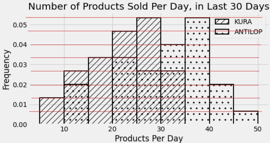
To find the number of days for which IKEA sold between 10 and 20 KURA reversible beds, we simply need to add the number of days in the [10, 15) and [15, 20) bins of the KURA distribution. Using the histogram with the red lines makes this easy to calculate as 4+5, or 9 days.
Therefore since 8<9<12, the correct answer is (2)<(3)<(1).
The average score on this problem was 81%.
On the graph paper below, draw the histogram that would be produced by this code.
(
sungod.take(np.arange(5))
      .plot(kind='hist', density=True,
      bins=np.arange(0, 7, 2), y='Appearance_Order');
)
In your drawing, make sure to label the height of each bar in the histogram on the vertical axis. You can scale the axes however you like, and the two axes don’t need to be on the same scale.
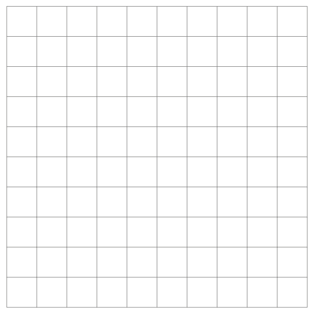
Answer:
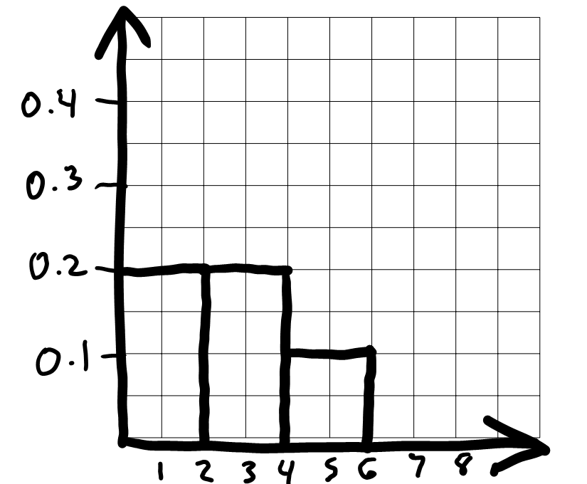
To draw the histogram, we first need to bin the data and figure out
how many data values fall into each bin. The code includes
bins=np.arange(0, 7, 2) which means the bin endpoints are
0, 2, 4, 6. This gives us three bins:
[0, 2), [2,
4), and [4, 6]. Remember that
all bins, except for the last one, include the left endpoint but not the
right. The last bin includes both endpoints.
Now that we know what the bins are, we can count up the number of
values in each bin. We need to look at the
'Appearance_Order' column of
sungod.take(np.arange(5)), or the first five rows of
sungod. The values there are 1,
4, 3, 1, 3. The two 1s fall into
the first bin [0, 2). The two 3s fall into the second bin [2, 4), and the one 4 falls into the last bin [4, 6]. This means the proportion of values
in each bin are \frac{2}{5}, \frac{2}{5},
\frac{1}{5} from left to right.
To figure out the height of each bar in the histogram, we use the fact that the area of a bar in a density histogram should equal the proportion of values in that bin. The area of a rectangle is height times width, so height is area divided by width.
For the bin [0, 2), the area is \frac{2}{5} = 0.4 and the width is 2, so the height is \frac{0.4}{2} = 0.2.
For the bin [2, 4), the area is \frac{2}{5} = 0.4 and the width is 2, so the height is \frac{0.4}{2} = 0.2.
For the bin [4, 6], the area is \frac{1}{5} = 0.2 and the width is 2, so the height is \frac{0.2}{2} = 0.1.
Since the bins are all the same width, the fact that there an equal number of values in the first two bins and half as many in the third bin means the first two bars should be equally tall and the third should be half as tall. We can use this to draw the rest of the histogram quickly once we’ve drawn the first bar.
The average score on this problem was 45%.
The histogram below displays the distribution of the number of Instagram followers each student has, measured in 100s. That is, if a student is represented in the first bin, they have between 0 and 200 Instagram followers.
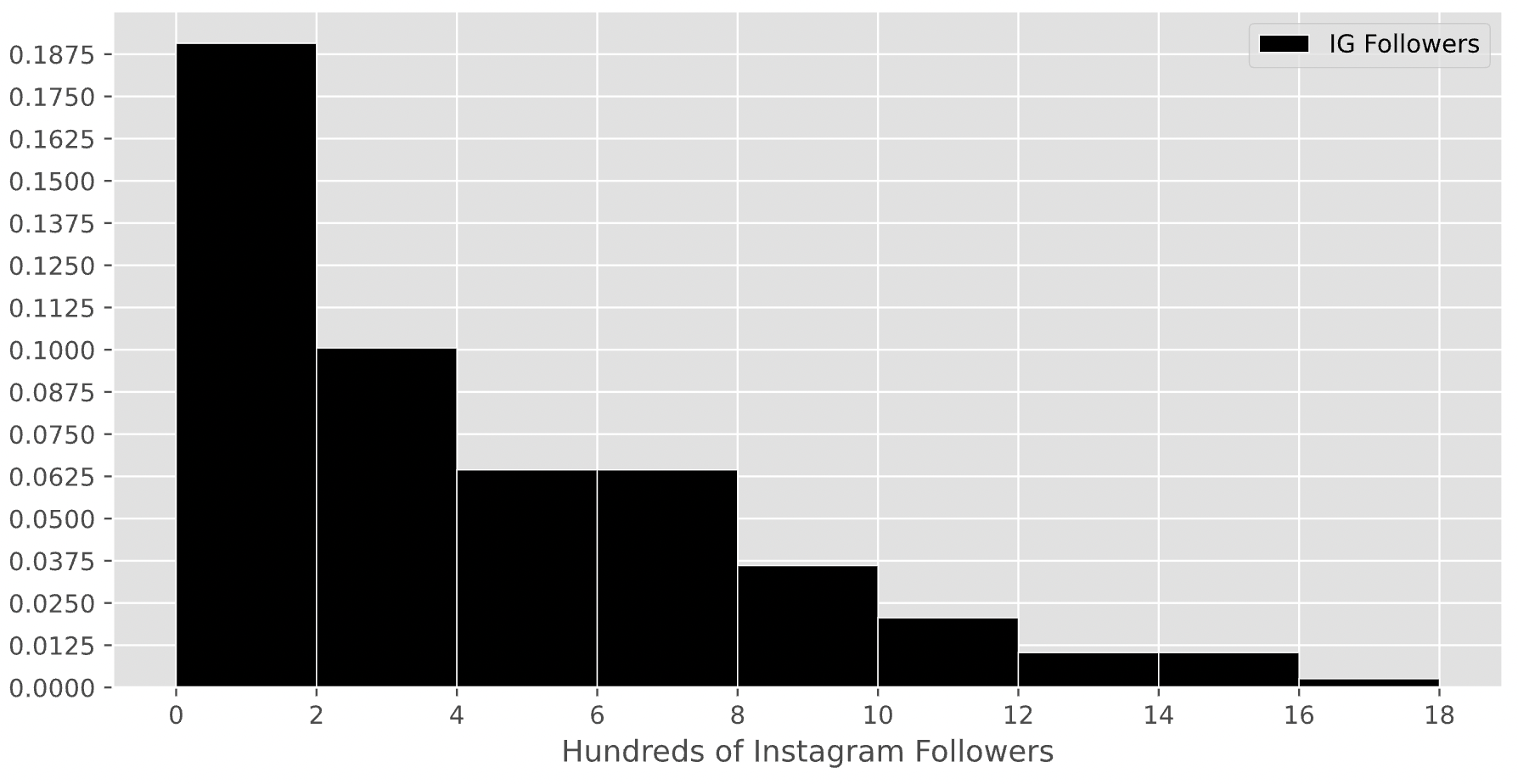
For this question only, assume that there are exactly 200 students in DSC 10.
How many students in DSC 10 have between 200 and 800 Instagram followers? Give your answer as an integer.
Answer: 90
Remember, the key property of histograms is that the proportion of values in a bin is equal to the area of the corresponding bar. To find the number of values in the range 2-8 (the x-axis is measured in hundreds), we’ll need to find the proportion of values in the range 2-8 and multiply that by 200, which is the total number of students in DSC 10. To find the proportion of values in the range 2-8, we’ll need to find the areas of the 2-4, 4-6, and 6-8 bars.
Area of the 2-4 bar: \text{width} \cdot \text{height} = 2 \cdot 0.1 = 0.2
Area of the 4-6 bar: \text{width} \cdot \text{height} = 2 \cdot 0.0625 = 0.125.
Area of the 6-8 bar: \text{width} \cdot \text{height} = 2 \cdot 0.0625 = 0.125.
Then, the total proportion of values in the range 2-8 is 0.2 + 0.125 + 0.125 = 0.45, so the total number of students with between 200 and 800 Instagram followers is 0.45 \cdot 200 = 90.
The average score on this problem was 49%.
Suppose the height of a bar in the above histogram is h. How many students are represented in the corresponding bin, in terms of h?
Hint: Just as in the first subpart, you’ll need to use the assumption from the start of the problem.
20 \cdot h
100 \cdot h
200 \cdot h
400 \cdot h
800 \cdot h
Answer: 400 \cdot h
As we said at the start of the last solution, the key property of histograms is that the proportion of values in a bin is equal to the area of the corresponding bar. Then, the number of students represented by a bar is the total number of students in DSC 10 (200) multiplied by the area of the bar.
Since all bars in this histogram have a width of 2, the area of a bar in this histogram is \text{width} \cdot \text{height} = 2 \cdot h. If there are 200 students in total, then the number of students represented in a bar with height h is 200 \cdot 2 \cdot h = 400 \cdot h.
To verify our answer, we can check to see if it makes sense in the context of the previous subpart. The 2-4 bin has a height of 0.1, and 400 \cdot 0.1 = 40. The total number of students in the range 2-8 was 90, so it makes sense that 40 of them came from the 2-4 bar, since the 2-4 bar takes up about half of the area of the 2-8 range.
The average score on this problem was 36%.
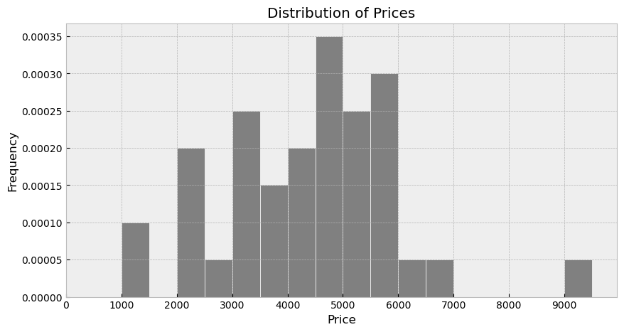
Yutian wants to rent a one-bedroom apartment, so she decides to learn
about the housing market by plotting a density histogram of the monthly
rent for all one-bedroom apartments in the apts DataFrame.
In her call to the DataFrame method .plot, she sets the
bins using the parameter
bins = np.arange(0, 10000, 100)
How many bins will this histogram have?
Answer: 99
np.arange(start, stop, step) takes the following three
parameters as arguments.
start: The starting value of the sequence
(inclusive).stop: The last value of the sequence (exclusive).step: The difference between each two consecutive
values.This means that np.arange(0, 10000, 100) will create a
NumPy array that starts at 0, and ends before it reaches 10000 - all
while incrementing by 100 for each step. To calculate the number of bins
within the parameter, we can write \frac{\text{stop} - \text{start}}{\text{step}} -
1.
Another way we can look at this is by taking a small sample of this
sequence (such as np.arange(0, 300, 100)). This will create
the array np.array([0, 100, 200]) without including the
stop argument (300). Note that the same equation holds true.
Note: Mathematically,
np.arange(start, stop) can be represented as [\text{start}, \text{stop})
The average score on this problem was 64%.
Suppose there are 300 one-bedroom apartments in the apts
DataFrame, and 15 of them cost between $2,300 (inclusive) and $2,400
(exclusive). How tall should the bar for the bin [2300, 2400) be in the density histogram?
Give your answer as a simplified fraction or exact decimal.
Answer: 0.0005 = \frac{1}{2000}
Before we start, we need to take note that the question is asking for the density of the bin, since we are representing the data in a density histogram. In order to calculate the density of the bin we use the following equation:
\frac{\text{Number of points in the bin}}{\text{Total number of points} \cdot \text{Width of bin}}
To solve, we plug in the following values into the equation:
\frac{15}{300 \cdot 100} = \frac{1}{20 \cdot 100} = \frac{1}{2000}
Therefore, the density of this bin is \frac{1}{2000}
The average score on this problem was 51%.
Suppose some of the one-bedroom apartments in the apts
DataFrame cost more than $5,000. Next, Yutian plots another density
histogram with
bins = np.arange(0, 5000, 100)
Consider the bin [2300, 2400) in
this new histogram. Is it taller, shorter, or the same height as in the
old histogram, where the bins were
np.arange(0, 10000, 100)?
Taller
Shorter
The same height
Not enough information to answer
Answer: Taller
In this histogram, we will only have data that that fits within the constraints of [0, 5000). Since we are told that there are apartments that fit outside of the constraint, there will be an overall smaller number of points points represented by the histogram.
Taking the histogram density estimation equation, \frac{\text{Number of points in the bin}}{\text{Total number of points} \cdot \text{Width of bin}}, we know that our total number of points have decreased (with respect to the constraints shown in the bins). So, a smaller denominator would lead to a proportional increase in the resulting product. Because the resulting product increases, this means that the height of this particular bin will be taller.
The average score on this problem was 55%.
Consider the histogram generated by the following code.
contacts.plot(kind="hist", y="Day", density=True, bins=np.arange(1, 33))Which of the following questions would you be able to answer from this histogram? Select all that apply.
How many of your contacts were born on a Monday?
How many of your contacts were born on January 1st?
How many of your contacts were born on the first day of the month?
How many of your contacts were born on the last day of the month?
Answer: Option 3: How many of your contacts were born on the first day of the month?
contacts.plot(kind="hist", y="Day", density=True, bins=np.arange(1, 33))
generates a histogram that visualizes the distribution of values in the
‘Day’ column of the contacts DataFrame.
bins=np.arange(1, 33) creates the bins
[1,2], [2,3], ..., [31,32]. Each bar in the histogram
represents the density of a day.
We can answer the question “How many of your contacts were born on the first day of the month?” by checking the bar containing the first day (the first bar).
However, the histogram doesn’t contain information of day of the week or month, so it can’t answer questions in options 1 or 2.
We also can’t choose option 4, because we have months with varying numbers of days (28, 29, 30, or 31). For months with 31 days, we know for sure it’s the last day of the month. For bars with 28, 29, and 30 days, we won’t be able to tell which proportion of days are the last day of the month since months with 31 days will have a count in all the previous number of days.
The average score on this problem was 80%.
After looking at the distribution of "Day" for your
contacts, you wonder how that distribution might look for other groups
of people.
In this problem, we will consider the distribution of day of birth (just the day of the month, not the month or year) for all babies born in the year 2023, under the assumption that all babies born in 2023 were equally likely to be born on each of the 365 days of the year.
The density histogram below shows this distribution.
Note: 2023 was not a leap year, so February had 28 days.
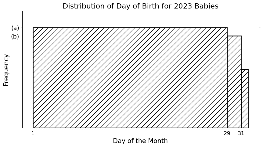
What is height (a)?
\dfrac{1}{28}
\dfrac{28}{365}
\dfrac{12 \cdot 28}{365}
\dfrac{1}{12}
\dfrac{12}{365}
1
Answer: \dfrac{12}{365}
2023 was not a leap year, so there are in total 365 days, and February only has 28 days. All the months have at least 28 days, so in bin [1,29], there are 12 * 28 data values. And, all the months other than February have 29th and 30th days, so there are 2 * 11 data values in bin [29,31]. Lastly, there are 7 months with 31 days, so there are 7 data values in bin [31,32].
There are in total 365 data values, so the proportion of data points falling into bin [1,29] =\dfrac{12 \cdot 28}{365}. Thus, the area of the bar of bin [1,29] = \dfrac{12 \cdot 28}{365}. Area = Height * Width, width of the bin is 28, so height(a) = \dfrac{12 \cdot 28}{365 \cdot 28} = \dfrac{12}{365}.
The average score on this problem was 38%.
Express height (b) in terms of height
(a).
\text{(b)} = \dfrac{7}{12} \cdot \text{(a)}
\text{(b)} = \dfrac{27}{28} \cdot \text{(a)}
\text{(b)} = \dfrac{28}{29} \cdot \text{(a)}
\text{(b)} = \dfrac{11}{12} \cdot \text{(a)}
\text{(b)} = \dfrac{7}{11} \cdot \text{(a)}
\text{(b)} = \dfrac{12 \cdot 28}{365} \cdot \text{(a)}
Answer: \text{(b)} = \dfrac{11}{12} \cdot \text{(a)}
Similarly, height(b) = \dfrac{2 \cdot 11}{365 \cdot 2} = \dfrac{11}{365} = \dfrac{11}{12} \cdot \dfrac{12}{365}.
The average score on this problem was 43%.
Which of the following correctly plots a density histogram showing
the distribution of "price" in art? Select all
that apply.
art.get(["price"]).plot(kind="hist", density=True)
art.get(["price"]).plot(kind="hist")
art.drop(columns=["artist", "year", "price"]).plot(kind="hist", density=True)
art.plot(kind="hist", y="price")
art.plot(kind="hist", y="price", density=True)
art.plot(kind="hist", x="price", density=True)
Answer: Options 1 and 5
The average score on this problem was 83%.
The density histogram below shows the distribution of
"price" in art. If the museum has 100 art
pieces in total, how many pieces cost at least $3,000 but less than
$4,500?
Answer: 30
The average score on this problem was 55%.
Below is a density histogram displaying the distribution of
reciprocal tariffs for each of the 50 countries on Trump’s chart. It was
plotted with the argument
bins=[10, 11, 15, 20, 40, 50].
Note that while the European Union is actually a group of many countries, it is counted as one country here.
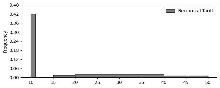
How many countries have a reciprocal tariff of 10%?
Answer: 21
Before attempting this problem, we must first understand how to interpret a density histogram. The x-axis represents the reciprocal tariff rate (in %), and the y-axis shows the density. The total area under the histogram sums to 1, with each bin corresponding to the proportion of countries falling within that bin.
The bins are defined as follows:
Countries with a reciprocal tariff of exactly 10% fall into the fist bin, [10, 11). The width of this bin is:
\text{width} = 11 - 10 = 1
Given that the height of the bin is 0.42, we calculate the area (i.e., the proportion of countries in this bin) using the formula:
\text{area} = \text{height} \times \text{width} \text{area} = .42 \times 1 \text{area} = .42
This, 42% of the countries fall within the [10, 11) range. If there are 50 countries in total, we compute the number of countries in this bin as:
50 \times .42 = 21
So, 21 countries have a reciprocal tariff rate between 10% and 11%.
The average score on this problem was 82%.
Suppose we plotted the same histogram, except we changed the
bins argument to
bins = [8, 15, 22, 30, 40, 50]. What would be the height of
the leftmost bar in this histogram? Give your answer as
a number to two decimal places.
Answer: 0.06
In this subproblem, we are told that the bins are changed. This time, instead of having a width of 1, the new bin has a width of 7 (15 - 8).
Looking back at the histogram given, we note that there is no data in the interval [11, 15); all the data within this new, wider bin comes from the previous [10, 11) bin.
We know the area is .42 as calculated in the prior subproblem, meaning all we have to do is recalculate the height using the changed width:
\text{area} = \text{height} \times \text{width} .42 = \text{height} \times 7 \frac{.42}{7} = \text{height} .06 = \text{height}
The average score on this problem was 52%.
The European Union is not actually one country, but a group of 27
countries. Imagine we were to replace the row of tariffs
corresponding to the European Union with 27 rows representing each of
the member countries (all with a 20\%
reciprocal tariff), then plot a histogram of the reciprocal tariffs
using bins = [10, 11, 15, 20, 40, 50].
Let h_{\text{new}} be the height of the rightmost bar in this histogram, and let h_{\text{old}} be the height of the rightmost bar in the original histogram shown above. Express h_{\text{new}} in terms of h_{\text{old}}.
Answer: h_{\text{new}} = \frac{50}{76} \cdot h_{\text{old}}
To solve this problem, we need to understand how modifying the dataset by replacing one row (The European Union) with 27 rows (each with a 20% reciprocal tariff) will affect the histogram: especially the rightmost bin, which is [40, 50].
In the original histograam, the number of total countries is 50. Now we can assume that the rightmost bin [40, 50] contains n countries. Since this is a density histogram, the height of a bin is given by:
\text{height} = \frac{\text{proportion of countries in bin}}{\text{width of bin}}
So, the original height of the rightmost bin is:
h_{\text{old}} = \frac{n}{50 \times 10}
Now, we change the dataset: instead of 50 countries, we now we have 76 countries (because we’re replacing 1 EU row with 27 separate rows, essentially adding 26, not 27 more entries).
The number of countries in the [40, 50] bin remains the same, in that none of the new EU entries fall into this bin (since they all have 20% tariff). However, the total number of countries increases, which affects the overall proportion.
The new height becomes: h_{\text{new}} = \frac{n}{76 \times 10}
Now, we divide the two to find h_{\text{new}} in terms of h_{\text{old}}:
\frac{h_{\text{new}}}{h_{\text{old}}} = \frac{n / (76 \times 10)}{n / (50 \times 10)} = \frac{50}{76}
\therefore h_{\text{new}} = \frac{50}{76} \cdot h_{\text{old}}
The average score on this problem was 19%.
Below is a density histogram showing the distribution of
"Runtime", in minutes, for all 25 films in ghibli.
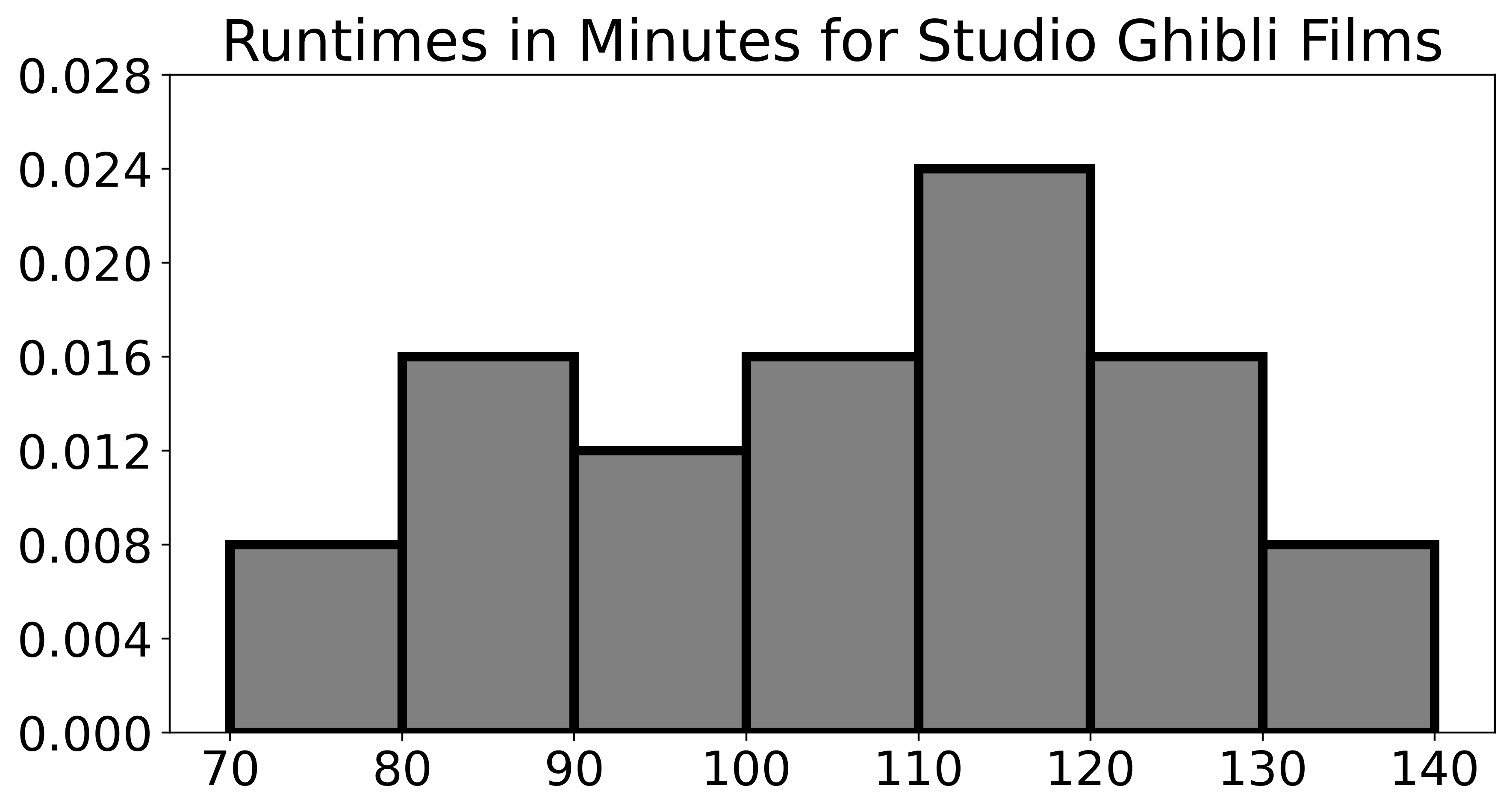
How many Studio Ghibli films are at least 90 minutes long?
Answer: 19
The average score on this problem was 79%.
Imagine we changed our histogram to have just one bin, from 70 to 140 minutes. What would the height of this bin be? Give your answer as an exact fraction or decimal.
Answer: \frac{1}{70}
The average score on this problem was 58%.
Below are two density histograms representing the distribution of Total Points for Division 1 and the distribution of Total Points for Division 2 teams (remember, there are six teams in each division):
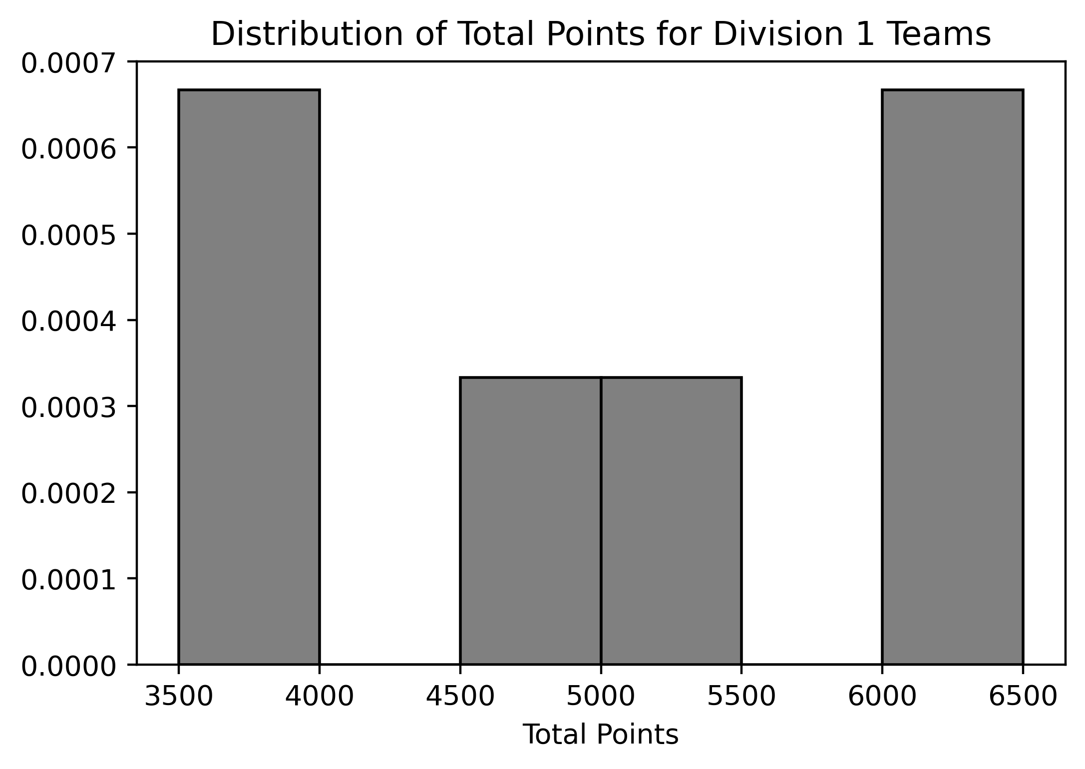
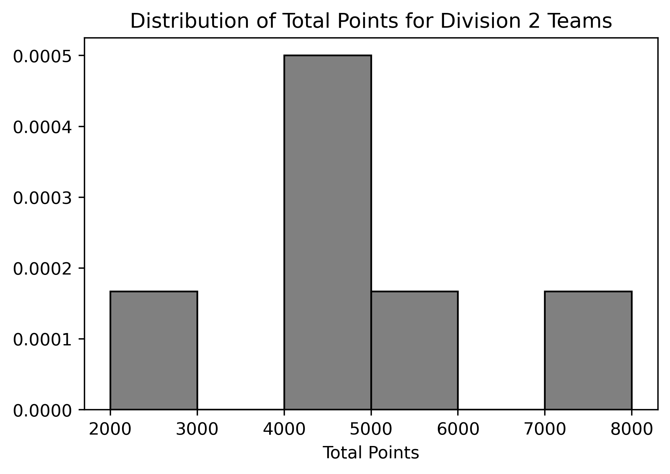
Assuming we know the bin values for each histogram, what can we conclude from these two histograms? Select all that apply:
The number of teams in the rightmost bin on the histogram that displays the distribution of total points for Division 2 teams.
The number of Division 1 teams that scored 4000 points.
The number of Division 2 teams that scored between 2000 and 3000 points.
The number of Division 2 teams that scored fewer points than the lowest-scoring Division 1 team.
Answer: Option 1, 2, 3, and 4
Since we are working with density histograms, each rectangle’s area represents the relative frequency of the corresponding bin. Given that there are six teams in each division, we can use the relative frequencies to approximate the number of teams in each bin.
[2000, 3000) bin in Division 2, we
can calculate the area of the bar and then multiply it by the total
number of teams (6) to estimate the number of teams that fall within
this range.[3500, 4000).
Division 2 has a bin that starts at a lower range
[2000, 3000), which is below Division 1’s minimum bin.
Therefore, we can determine the number of Division 2 teams that scored
fewer points than the lowest-scoring Division 1 team.
The average score on this problem was 85%.
Suppose that we changed the histogram of total points for Division 2
teams so that the bins were
[2000, 4000), [4000, 6000), [6000, 8000). If the bin
defined by [2000, 4000) contained one team, as it does in
the original graph, what would the height of the middle bar (with bin
[4000, 6000)) be? Do not simplify your answer.
Answer: \frac{1}{3000}
First, we need to calculate the number of teams that scored in the
range of [4000,6000) in the original histogram for Division
2 teams:
Area of bar in bin[4000, 5000) * 6 + Area of bar in
bin[5000, 6000) * 6 = 0.0005 * 1000 * 6 + 0.00017 * 1000 *
6 = 4.02
Rounding to the nearest whole number, we find that approximately 4 teams fall within this range.
Next, we want to calculate the height of the bar with bin
[4000, 6000) in the new histogram. Using the fact that this
bin should contain 4 teams, we have:
Height * Width * 6 = 4
Solving for the height:
Height = 4 / (6 * 2000) = \frac{1}{3000}
The average score on this problem was 64%.
Suppose we drew different bins for the histogram of total points for
Division 2 teams. If the bin defined by [2000, 4000)
contained one team, as it does in the original graph, and the bin
defined by [4000, 4500) contained two teams, what would the
height of the bar with bin [4500, 5000) be? Do not simplify
your answer.
Answer: \frac{1}{3000}
In the original histogram, the bin defined by
[4000, 5000) contained: 0.0005 * 1000 * 6 = 3 teams
According to the description, the bin defined by
[4000, 4500) contained 2 teams.
Therefore, we can conclude that the bin defined by
[4500, 5000) contained: 3 - 2 = 1 team
In the bin [4500, 5000) of the new histogram, we have:
Height * Width * 6 = 1
Solving for the height: Height = 1 / (6 * Width) = 1 / (6 * 500) = \frac{1}{3000}
The average score on this problem was 32%.
Suppose you have a dataset of 29 art galleries that includes the number of pieces of art in each gallery.
A histogram of the number of art pieces in each gallery, as well as the code that generated it, is shown below.
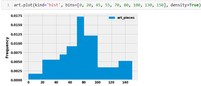
How many galleries have at least 80 but less than 100 art pieces? Input your answer below. Make sure your answer is an integer and does not include any text or symbols.
Answer: 7
Through looking at the graph we can find the total number of art galleries by taking 0.012 (height of bin) * 20 (the size of the bin) * 29 (total number of art galleries). This will yield an anwser of 6.96 which should be rounded to the nearest integer (7).
The average score on this problem was 94%.
If we added to our dataset two more art galleries, each containing 24
pieces of art, and plotted the histogram again for the larger dataset,
what would be the height of the bin [20,45)? Input your
answer as a number rounded to six decimal places.
Answer: 0.007742
Taking the area of the bin [20,45] we can find the
number of art galleries already within this bin 0.0055 * 25 = 0.1375
(estimation based on the visualization). To find the number take this
proportion x the total number of art galleries. 0.1375 * 29 = about 4
art galleries. If we add two art galleries to this total we get 4 art
galleries in the [20,45] bin to get 6 art galleries. To
find the frequency of 6 art galleries to the entire data set we can take
6/31. Note that the question asks for the height of the bin.
Therefore, we can take (6/31) / 25 due to the size of the bin which will
give an answer of 0.007742 upon rounding to six decimal places.
The average score on this problem was 66%.
You have a DataFrame called prices that contains
information about food prices at 18 different grocery stores. There is
column called 'broccoli' that contains the price in dollars
for one pound of broccoli at each grocery store. There is also a column
called 'ice_cream' that contains the price in dollars for a
pint of store-brand ice cream.
What should type(prices.get('broccoli').iloc[0])
output?
int
float
array
Series
Answer: float
This code extracts the first entry of the 'broccoli'
column. Since this column contains prices in dollars for a pound of
broccoli, it makes sense to represent such a price using a float,
because the price of a pound of broccoli is not necessarily an
integer.
The average score on this problem was 92%.
Using the code,
prices.plot(kind='hist', y='broccoli', bins=np.arange(0.8, 2.11, 0.1), density=True)we produced the histogram below:
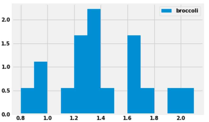
How many grocery stores sold broccoli for a price greater than or equal to $1.30 per pound, but less than $1.40 per pound (the tallest bar)?
Answer: 4 grocery stores
We are given that the bins start at 0.8 and have a width of 0.1, which means one of the bins has endpoints 1.3 and 1.4. This bin (the tallest bar) includes all grocery stores that sold broccoli for a price greater than or equal to $1.30 per pound, but less than $1.40 per pound.
This bar has a width of 0.1 and we’d estimate the height to be around 2.2, though we can’t say exactly. Multiplying these values, the area of the bar is about 0.22, which means about 22 percent of the grocery stores fall into this bin. There are 18 grocery stores in total, as we are told in the introduction to this question. We can compute using a calculator that 22 percent of 18 is 3.96. Since the actual number of grocery stores this represents must be a whole number, this bin must represent 4 grocery stores.
The reason for the slight discrepancy between 3.96 and 4 is that we used 2.2 for the height of the bar, a number that we determined by eye. We don’t know the exact height of the bar. It is reassuring to do the calculation and get a value that’s very close to an integer, since we know the final answer must be an integer.
The average score on this problem was 71%.
Suppose we now plot the same data with different bins, using the following line of code:
prices.plot(kind='hist', y='broccoli', bins=[0.8, 1, 1.1, 1.5, 1.8, 1.9, 2.5], density=True)What would be the height on the y-axis for the bin corresponding to the interval [\$1.10, \$1.50)? Input your answer below.
Answer: 1.25
First, we need to figure out how many grocery stores the bin [\$1.10, \$1.50) contains. We already know from the previous subpart that there are four grocery stores in the bin [\$1.30, \$1.40). We could do similar calculations to find the number of grocery stores in each of these bins:
However, it’s much simpler and faster to use the fact that when the bins are all equally wide, the height of a bar is proportional to the number of data values it contains. So looking at the histogram in the previous subpart, since we know the [\$1.30, \$1.40) bin contains 4 grocery stores, then the [\$1.10, \$1.20) bin must contain 1 grocery store, since it’s only a quarter as tall. Again, we’re taking advantage of the fact that there must be an integer number of grocery stores in each bin when we say it’s 1/4 as tall. Our only options are 1/4, 1/2, or 3/4 as tall, and among those choices, it’s clear.
Therefore, by looking at the relative heights of the bars, we can quickly determine the number of grocery stores in each bin:
Adding these numbers together, this means there are 9 grocery stores whose broccoli prices fall in the interval [\$1.10, \$1.50). In the new histogram, these 9 grocery stores will be represented by a bar of width 1.50-1.10 = 0.4. The area of the bar should be \frac{9}{18} = 0.5. Therefore the height must be \frac{0.5}{0.4} = 1.25.
The average score on this problem was 33%.
You are interested in finding out the number of stores in which a pint of ice cream was cheaper than a pound of broccoli. Will you be able to determine the answer to this question by looking at the plot produced by the code below?
prices.get(['broccoli', 'ice_cream']).plot(kind='barh')Yes
No
Answer: Yes
When we use .plot without specifying a y
column, it uses every column in the DataFrame as a y column
and creates an overlaid plot. Since we first use get with
the list ['broccoli', 'ice_cream'], this keeps the
'broccoli' and 'ice_cream' columns from
prices, so our bar chart will overlay broccoli prices with
ice cream prices. Notice that this get is unnecessary
because prices only has these two columns, so it would have
been the same to just use prices directly. The resulting
bar chart will look something like this:
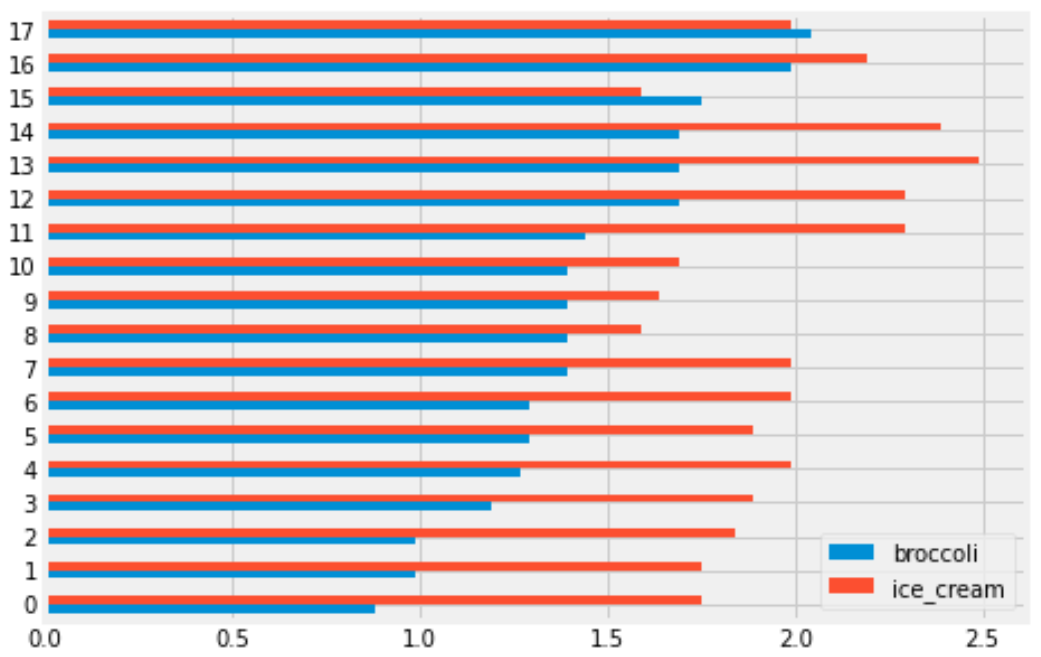
Each grocery store has its broccoli price represented by the length of the blue bar and its ice cream price represented by the length of the red bar. We can therefore answer the question by simply counting the number of red bars that are shorter than their corresponding blue bars.
The average score on this problem was 78%.
You are interested in finding out the number of stores in which a pint of ice cream was cheaper than a pound of broccoli. Will you be able to determine the answer to this question by looking at the plot produced by the code below?
prices.get(['broccoli', 'ice_cream']).plot(kind='hist')Yes
No
Answer: No
This will create an overlaid histogram of broccoli prices and ice cream prices. So we will be able to see the distribution of broccoli prices together with the distribution of ice cream prices, but we won’t be able to pair up particular broccoli prices with ice cream prices at the same store. This means we won’t be able to answer the question. The overlaid histogram would look something like this:
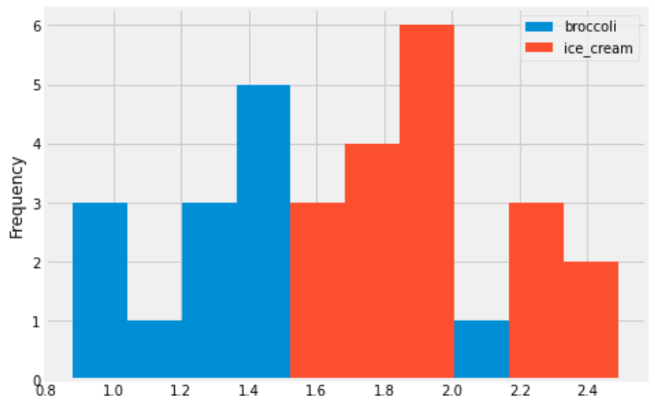
This tells us that broadly, ice cream tends to be more expensive than broccoli, but we can’t say anything about the number of stores where ice cream is cheaper than broccoli.
The average score on this problem was 81%.
Some code and the scatterplot that produced it is shown below:
(prices.get(['broccoli', 'ice_cream']).plot(kind='scatter', x='broccoli', y='ice_cream'))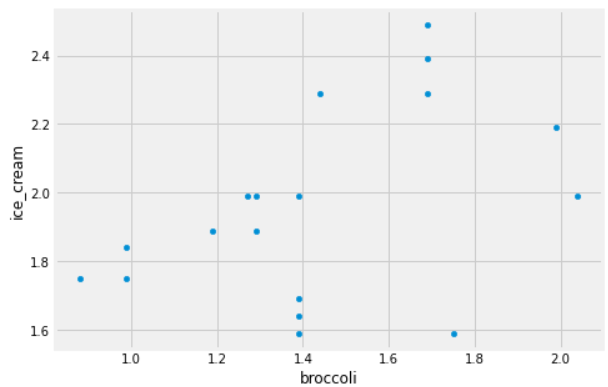
Can you use this plot to figure out the number of stores in which a pint of ice cream was cheaper than a pound of broccoli?
If so, say how many such stores there are and explain how you came to that conclusion.
If not, explain why this scatterplot cannot be used to answer the question.
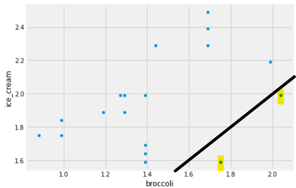
Answer: Yes, and there are 2 such stores.
In this scatterplot, each grocery store is represented as one dot. The x-coordinate of that dot tells the price of broccoli at that store, and the y-coordinate tells the price of ice cream. If a grocery store’s ice cream price is cheaper than its broccoli price, the dot in the scatterplot will have y<x. To identify such dots in the scatterplot, imagine drawing the line y=x. Any dot below this line corresponds to a point with y<x, which is a grocery store where ice cream is cheaper than broccoli. As we can see, there are two such stores.
The average score on this problem was 78%.
You are given a DataFrame called restaurants that
contains information on a variety of local restaurants’ daily number of
customers and daily income. There is a row for each restaurant for each
date in a given five-year time period.
The columns of restaurants are 'name'
(string), 'year' (int), 'month' (int),
'day' (int), 'num_diners' (int), and
'income' (float).
Assume that in our data set, there are not two different restaurants
that go by the same 'name' (chain restaurants, for
example).
What type of visualization would be best to display the data in a way that helps to answer the question “Do more customers bring in more income?”
scatterplot
line plot
bar chart
histogram
Answer: scatterplot
The number of customers is given by 'num_diners' which
is an integer, and 'income' is a float. Since both are
numerical variables, neither of which represents time, it is most
appropriate to use a scatterplot.
The average score on this problem was 87%.
What type of visualization would be best to display the data in a way that helps to answer the question “Have restaurants’ daily incomes been declining over time?”
scatterplot
line plot
bar chart
histogram
Answer: line plot
Since we want to plot a trend of a numerical quantity
('income') over time, it is best to use a line plot.
The average score on this problem was 95%.
Recall, the interval [a, b) refers to numbers greater than or equal to a and less than b, and the interval [a, b] refers to numbers greater than or equal to a and less than or equal to b.
Suppose we created a DataFrame, medium_sky, containing
only the skyscrapers in sky whose number of floors are in
the interval [20, 60]. Below, we’ve
drawn a histogram of the number of floors of all skyscrapers in
medium_sky.
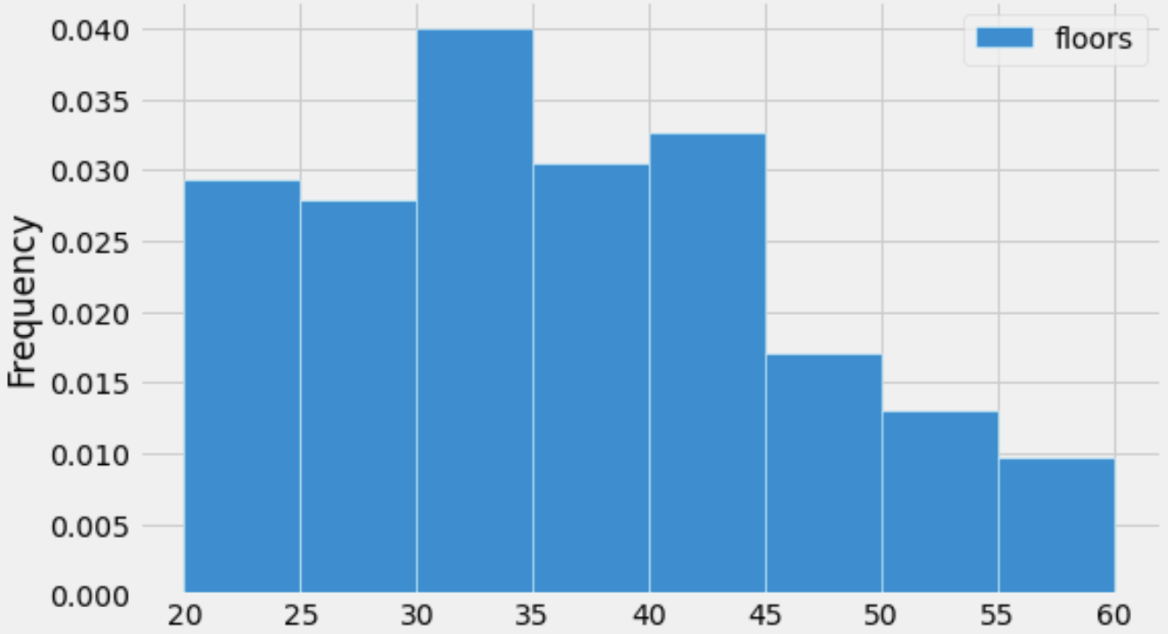
Suppose that there are 160 skyscrapers whose number of floors are in the interval [30, 35).
Given this information and the histogram above, how many skyscrapers
are there in medium_sky?
Answer: 800
Recall, in a histogram,
\text{proportion of values in bin} = \text{area of bar} = \text{width of bin} \cdot \text{height of bar}
Also, note that:
\text{\# of values satisfying condition} = \text{proportion of values satisfying condition} \cdot \text{total \# of values}
Here, we’re given the entire histogram, so we can find the proportion
of values in the [30, 35) bin. We are
also given the number of values in the [30,
35) bin (160). This means we can use the second equation above to
find the total number of skyscrapers in medium_sky.
The first step is finding the area of the [30, 35) bin’s bar. Its width is 35-30 = 5, and its height is 0.04, so its area is 5 \cdot 0.04 = 0.2. Then,
\begin{aligned} \text{\# of values satisfying condition} &= \text{proportion of values satisfying condition} \cdot \text{total \# of values} \\ 160 &= 0.2 \cdot \text{total \# of values} \\ \implies \text{total \# of values} &= \frac{160}{0.2} = 160 \cdot 5 = 800 \end{aligned}
The average score on this problem was 62%.
Again, suppose that there are 160 skyscrapers whose number of floors are in the interval [30, 35).
Now suppose that there is a typo in the medium_sky
DataFrame, and 20 skyscrapers were accidentally listed as having 53
floors each when instead they actually only have 35 floors each. The
histogram drawn above contains the incorrect version of the data.
Suppose we re-draw the above histogram using the correct data. What will be the new heights of both the [35, 40) bar and [50, 55) bar? Select the closest answer.
The [35, 40) bar’s height becomes 0.0325, and the [50, 55) bar’s height becomes 0.0105.
The [35, 40) bar’s height becomes 0.035, and the [50, 55) bar’s height becomes 0.008.
The [35, 40) bar’s height becomes 0.0375, and the [50, 55) bar’s height becomes 0.0055.
The [35, 40) bar’s height becomes 0.04, and the [50, 55) bar’s height becomes 0.003.
Answer: The [35, 40) bar’s height becomes 0.035, and the [50, 55) bar’s height becomes 0.008.
The current height of the [35, 40) bar is 0.03, and the current height of the [50, 55) bar is 0.013 (approximately; its height appears to be slightly more than halfway between 0.01 and 0.015). We need to decrease the height of the [50, 55) bar and increase the height of the [35, 40) bar. The combined area of both bars must stay the same, since the proportion of values in their bins (together) is not changing. This means that the amount we need to decrease the [50, 55) bar’s height by is the same as the amount we need to increase the [35, 40) bar’s height by. Note that this relationship is true in all 4 answer choices.
In the question, we were told that 20 skyscrapers were incorrectly binned. There are 800 skyscrapers total, so the proportion of skyscrapers that were incorrectly binned is \frac{20}{800} = 0.025. This means that the area of the [35, 40) bar needs to increase by 0.025 and the area of the [50, 55) bar needs to decrease by 0.025. Recall, each bar has width 5. That means that the “rectangular section” we will add to the [35, 40) bar and remove from the [50, 55) bar has height
\text{height} = \frac{\text{area}}{\text{width}} = \frac{0.025}{5} = 0.005
Thus, the height of the [35, 40) bar becomes 0.03 + 0.005 = 0.035 and the height of the [50, 55) bar becomes 0.013 - 0.005 = 0.008.
The average score on this problem was 74%.
Consider the following line plot, which depicts the number of skyscrapers built per year.
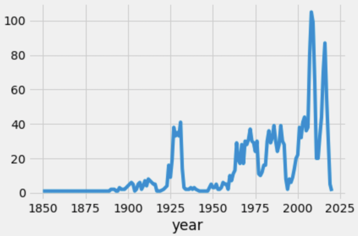
We created the line plot above using the following line of code:
sky.groupby('year').count().plot(kind='line', y='height');Which of the following could we replace 'height' with in
the line of code above, such that the resulting line of code creates the
same line plot? Select all that apply.
'name'
'material'
'city'
'floors'
'year'
None of the above
Answers: 'material',
'city', and 'floors'
Recall that when we use the .count() aggregation method
while grouping, the values in all resulting columns are the same (they
all contain the number of values in each unique group). This means that
any column of sky.groupby('year').count() can replace
'height' in the provided line.
'name' is not a column in
sky.groupby('year').count(). 'name' was the
index in sky, but is not present at all in
sky.groupby('year').count() (the original index is lost
completely). 'year' is also not a column in
sky.groupby('year').count(), since it is the index. The
remaining three columns – 'material', 'city',
and 'floors' – would all work.
The average score on this problem was 74%.
Note: This problem is out of scope; it covers material no longer included in the course.
Now let’s look at the number of skyscrapers built each year since 1975 in New York City 🗽.
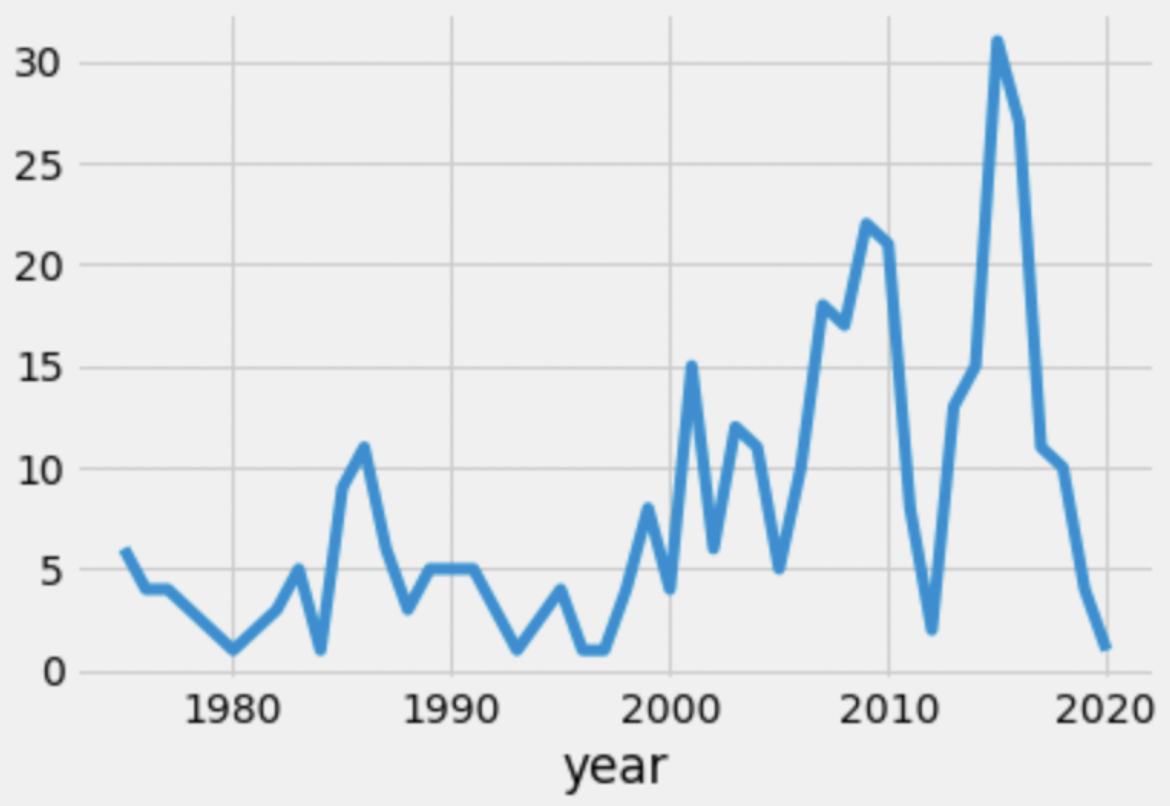
Which of the following is a valid conclusion we can make using this graph alone?
No city in the dataset had more skyscrapers built in 2015 than New York City.
The decrease in the number of skyscrapers built in 2012 over previous years was due to the 2008 economic recession, and the reason the decrease is seen in 2012 rather than 2008 is because skyscrapers usually take 4 years to be built.
The decrease in the number of skyscrapers built in 2012 over previous years was due to something other than the 2008 economic recession.
The COVID-19 pandemic is the reason that so few skyscrapers were built in 2020.
None of the above.
Answer: None of the above.
Let’s look at each answer choice.
Tip: This is a typical “cause-and-effect” problem that you’ll see in DSC 10 exams quite often. In order to establish that some treatment had an effect, we need to run a randomized controlled trial, or have some other guarantee that there is no difference between the naturally-observed control and treatment groups.
The average score on this problem was 90%.
In which of the following scenarios would it make sense to draw a overlaid histogram?
To visualize the number of skyscrapers of each material type, separately for New York City and Chicago.
To visualize the distribution of the number of floors per skyscraper, separately for New York City and Chicago.
To visualize the average height of skyscrapers built per year, separately for New York City and Chicago.
To visualize the relationship between the number of floors and height for all skyscrapers.
Answer: To visualize the distribution of the number of floors per skyscraper, separately for New York City and Chicago.
Recall, we use a histogram to visualize the distribution of a numerical variable. Here, we have a numerical variable (number of floors) that is split across two categories (New York City and Chicago), so we need to draw two histograms, or an overlaid histogram.
In the three incorrect answer choices, another visualization type is more appropriate. Given the descriptions here, see if you can draw what each of these three visualizations should look like.
The average score on this problem was 62%.
Suppose males is a DataFrame of all male Olympic
weightlifting medalists with a column called "Weight"
containing their body weight. Similarly, females is a
DataFrame of all female Olympic weightlifting medalists. It also has a
"Weight" column with body weights.
The males DataFrame has 425 rows and
the females DataFrame has 105 rows, since
women’s weightlifting became an Olympic sport much later than men’s.
Below, density histograms of the distributions of
"Weight" in males and females are
shown on the same axes:
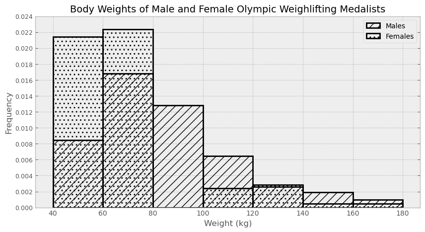
Estimate the number of males included in the third bin (from 80 to 100). Give your answer as an integer, rounded to the nearest multiple of 10.
Answer: 110
We can estimate the number of males included in the third bin (from 80 to 100) by multiplying the area of that particular histogram bar by the total number of males. The bar has a height of around 0.013 and a width of 20, so the bar has an area of 0.013 \cdot 20 = 0.26, which means 26% of males fall in that bin. Since there are 425 total males, 0.26 \cdot 425 ≈ 110 males are in that bin, rounded to the nearest multiple of 10.
The average score on this problem was 81%.
Using the males DataFrame, write one line of code that
evaluates to the exact number of males included in the third bin (from
80 to 100).
Answer:
males[(males.get("Weight")>=80) & (males.get("Weight")<100)].shape[0]
To get the exact number of males in the third bin (from 80 to 100)
using code, we can query the males DataFrame to only include rows where
"Weight" is greater than or equal to 80, and
"Weight" is less than 100. Remember, a histogram bin
includes the lower bound (in this case, 80) and excludes the upper bound
(in this case, 100). Remember to put parentheses around each condition,
or else the order of operations will change your intended conditions.
After querying, we use .shape[0] to get the number of rows
in that dataframe, therefore getting the number of males with a weight
greater than or equal to 80, and less than 100.
The average score on this problem was 75%.
Among Olympic weightlifting medalists who weigh less than 60 kilograms, what proportion are male?
less than 0.25
between 0.25 and 0.5
between 0.5 and 0.75
more than 0.75
Answer: between 0.5 and 0.75
We can answer this question by calculating the approximate number of males and females in the first bin (from 40 to 60). Be careful, we cannot simply compare the areas of the bars because the number of male weightlifting medalists is different from the number of female weightlifting medalists. The approximate number of male weightlifting medalists is equal to 0.008 \cdot 20 \cdot 425 = 68, while the approximate number of female weightlifting medalists is equal to 0.021 \cdot 20 \cdot 105 = 44. The proportion of male weightlifting medalists who weigh less than 69 kg is approximately \frac{68}{68 + 44} = 0.607, which falls in the category of “between 0.5 and 0.75”.
The average score on this problem was 54%.
The histogram below shows the distribution of game times in minutes for both two-player and three-player games of Clue, with each distribution representing 1000 games played.
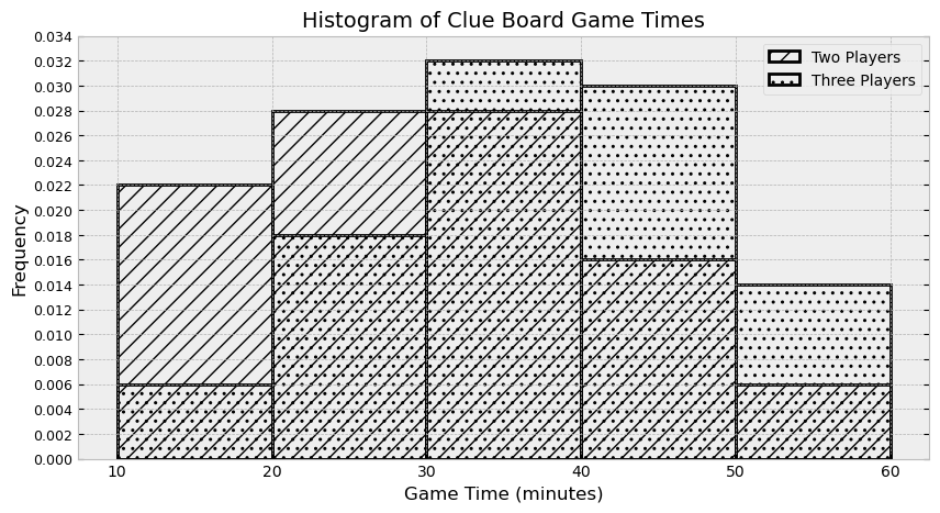
How many more three-player games than two-player games took at least 50 minutes to play? Give your answer as an integer, rounded to the nearest multiple of 10.
Answer: 80
First, calculate the number of three-player games that took at least 50 minutes. We can calculate this number by multiplying the area of that particular histogram bar (from 50 to 60) by the total number of three player games(1000 games) total. This results in (60-50) \cdot 0.014 \cdot 1000 = 140. We repeat the same process to find the number of two-player games that took at least 50 minutes, which is (60-50) \cdot 0.006 \cdot 1000 = 60. Then, we find the difference of these numbers, which is 140 - 60 = 80.
An easier way to calculate this is to measure the difference directly. We could do this by finding the area of the highlighted region below and then multiplying by the number of games. This represents the difference between the number of three-player games and the number of two player games. This, way we need to do just one calculation to get the same answer: (60 - 50) \cdot (0.014 - 0.006) \cdot 1000 = 80.
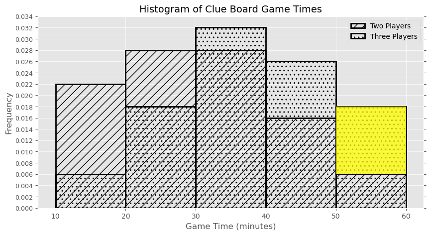
The average score on this problem was 61%.
Calculate the approximate area of overlap of the two histograms. Give your answer as a proportion between 0 and 1, rounded to two decimal places.
Answer: 0.74
To find the area of overlap of the two histograms, we can directly calculate the area of overlap in each bin and add them up as shown below. However, this requires a lot of calculation, and is not advised.
From 10-20: (20-10) \cdot 0.006 = 0.06
From 20-30: (30-20) \cdot 0.018 = 0.18
From 30-40: (40-30) \cdot 0.028 = 0.28
From 40-50: (50-40) \cdot 0.016 = 0.16
From 50-60: (60-50) \cdot 0.006 = 0.06
The summation of the overlap here is 0.74!
A much more efficient way to do this problem is to find the area of overlap by taking the total area of one distribution (which is 1) and subtracting the area in that distribution that does not overlap with the other. In the picture below, the only area in the two-player distribution that does not overlap with three-player distribution is highlighted. Notice there are only two regions to find the area of, so this is much easier. The calculation comes out the same: 1 - ((20 - 10) \cdot (0.022-0.006) + (30 - 20) \cdot (0.028 - 0.018) = 0.74.
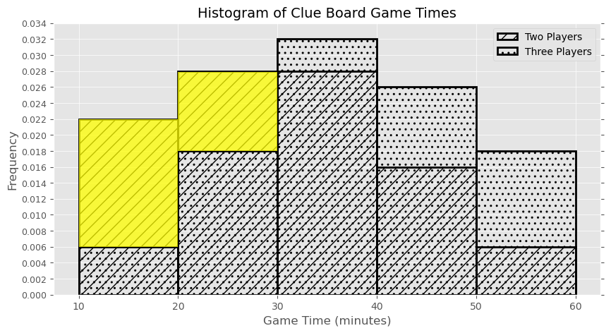
The average score on this problem was 56%.
Select all the true statements below.
When you set the index of a DataFrame, the specified column becomes the index, and the old index becomes a column.
After grouping a DataFrame, the resulting number of rows is less than or equal to the original number of rows.
The area of a density histogram is always equal to 1.
A scatter plot has one numerical axis and one categorical axis.
The height of the tallest bar in a density histogram is always less than 1.
Answer: Option 2 and Option 3
The average score on this problem was 84%.
A density histogram of "Screen Size" is shown below.
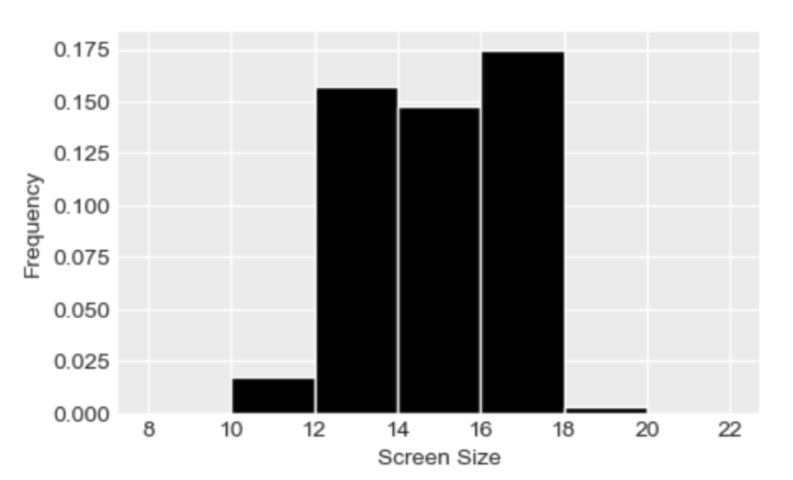
What percentage of computer models have a
"Screen Size" of at least 16 inches but less than 18
inches? Give your answer as an integer rounded to the nearest
multiple of 5.
Answer 35%
The average score on this problem was 72%.
Below is a density histogram displaying the distribution of wait times for orders from UCSD dining halls.
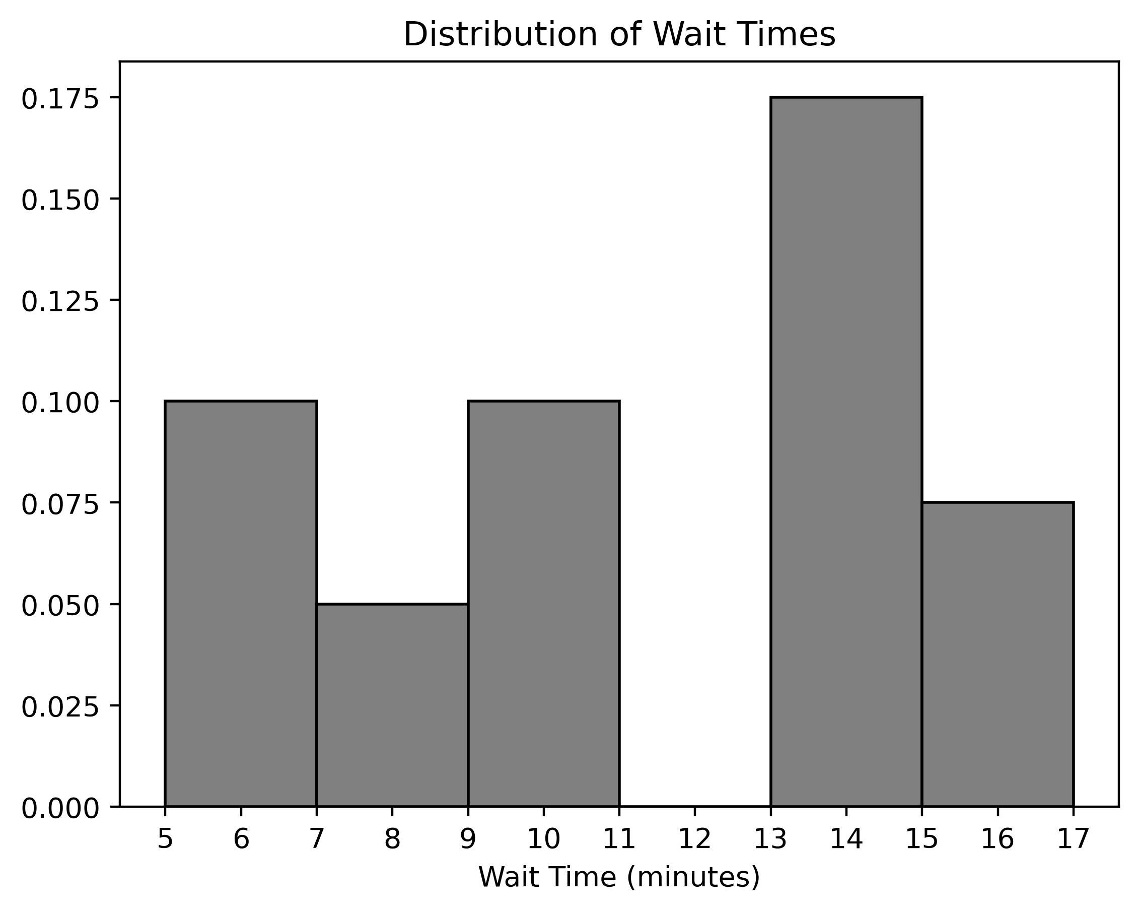
Fill in the blanks to define a variable bins that could
have been used as the bins argument in the call to
.plot that generated the histogram above.
bins = 0.5 * (2 + np.arange(__(a)__, __(b)__, __(c)__))Answer (a): 8
The first piece of information to note is what the bins are in the
original histogram; if we know where we need to arrive at the end of the
problem, it is much easier to piece together the arguments we need to
pass to np.arange in the code provided.
With this in mind, the bins in the original histogram are defined by
the array with values [5, 7, 9, 11, 13, 15, 17]. So, we can
work backwards from here to answer this question.
The final step in the code is multiplying the result of
2 + np.arange(a, b, c) by 0.5. Since we know
this must result in [5, 7, 9, 11, 13, 15, 17], the array
generated by 2 + np.arange(a, b, c) must have the values
[10, 14, 18, 22, 26, 30, 34].
Using similar logic, we know that 2 + np.arange(a, b, c)
must give us the array with values
[10, 14, 18, 22, 26, 30, 34]. By subtracting two, we get
that np.arange(a, b, c) must have values
[8, 12, 16, 20, 24, 28, 32].
There are multiple calls to np.arange() that result in
this sequence. We should start at 8 and step by
4, but where we stop can be any number larger than
32, and at most 36, as this argument is
exclusive and not included in the output array. So, the answers are (a)
= 8, (b) = any number larger than 32 and less
than or equal to 36, and (c) = 4.
The average score on this problem was 68%.
Answer (b): any number in the interval
(32, 36]
Refer to explanation for (a).
The average score on this problem was 56%.
Answer (c): 4
Refer to explanation for (a).
The average score on this problem was 36%.
What proportion of orders took at least 7 minutes but less than 12 minutes to complete?
Answer: 0.3 or 30%
In a density histogram, the proportion of data in a bar or set of bars is equal to the area of those bars. So, to find the proportion of orders that took between 7 and 12 minutes to complete, we must find the area of the bars that encapsulate this range.
The bars associated with the bins [7, 9) and [9, 11) contain all of the orders that took between 7 and 12 minutes. So, summing the areas of these bars tells us the proportion of orders that took between 7 and 12 minutes.
The width of each bar is 2, and the heights of the bars are 0.05 and 0.1, respectively. So, the sum of their areas is 2 \cdot 0.05 + 2 \cdot 0.1 = 0.1 + 0.2 = 0.3. So, 0.30 or 30\% of our orders took between 7 and 12 minutes to complete.
The average score on this problem was 82%.
After some investigation, HDH discovers that every order that took longer than 12 minutes to complete was ordered from The Bistro. As a result, they fire all the employees at The Bistro and permanently close the dining hall. With this update, we generate a new density histogram displaying the distribution of wait times for orders from the other UCSD dining halls.
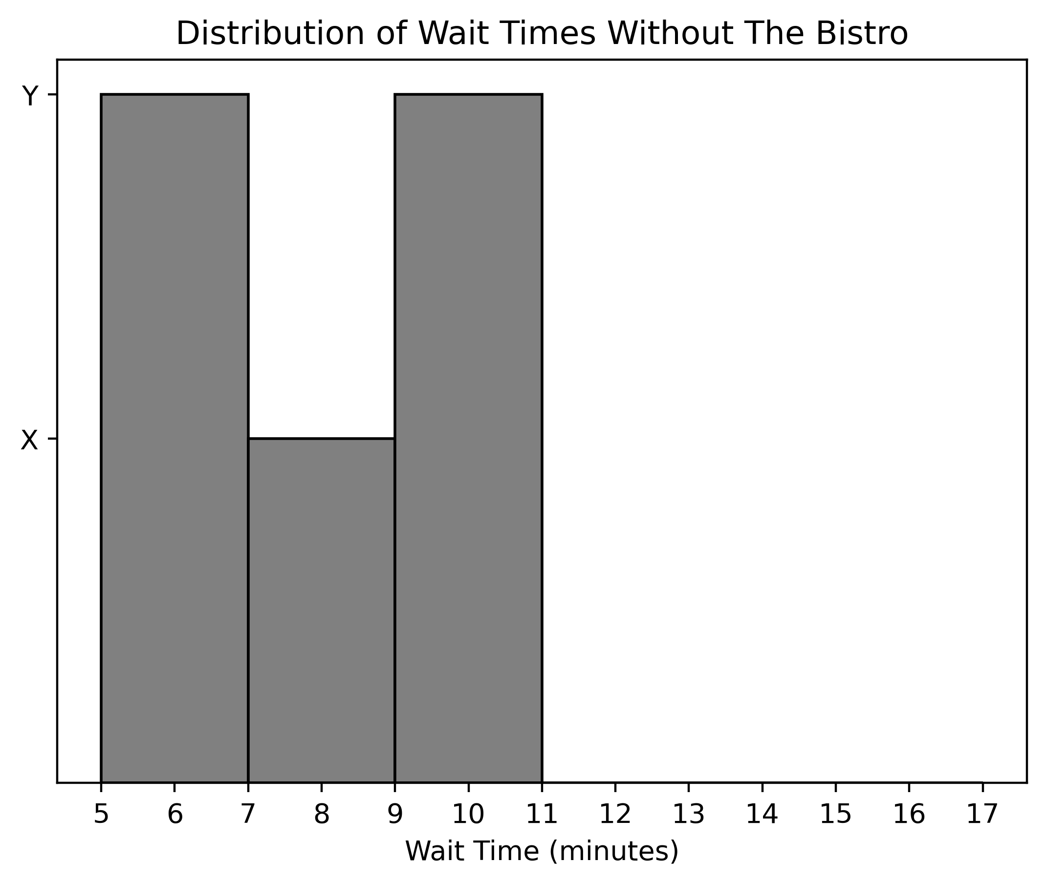
What are the values of X and Y along the y-axis of this histogram?
Answer: X = 0.1, Y = 0.2
The original histogram, including The Bistro’s data, showed a
cumulative density of 0.5 for the first three bars covering
wait times from 5 to 11 minutes. The densities were calculated as:
After we removed The Bistro’s data, these wait time intervals (5 to
11 minutes) now account for the entirety of the dataset. Hence, to
reflect the new total (100% of the data), the original bar heights need
to be doubled, as they previously summed up to 0.5 (or 50%
of the data).
Thus, the new calculation for total density is: 2 \times 0.2 + 2 \times 0.1 + 2 \times 0.2 = 1.0.
The average score on this problem was 53%.
The density histogram below shows the distribution of
"num_toppings" for 250 unique orders in
blue_bowl.
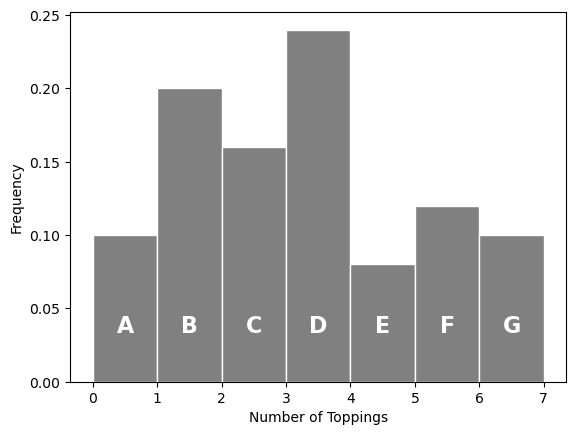
Kate orders a bowl with exactly two toppings. Which bin is her order included in?
A
B
C
D
E
F
G
Answer: C
The average score on this problem was 89%.
How many more orders were there with one topping than orders with no toppings? Give your answer as an integer rounded to the nearest multiple of 5.
Answer: 25
The average score on this problem was 81%.
The distribution of prices in orders is
summarized by the histogram below. If the cafe sold 700 drinks with a
price less than 6 dollars, how many drinks did the cafe
sell in total?
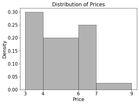
Answer: 1000 drinks.
The histogram is a density histogram, so the area of each bar is the proportion of orders in that price range.
So the proportion with price strictly less than 6 dollars is 0.30 + 0.40 = 0.70.
If 700 drinks correspond to 70% of the data, the total number of drinks is 700 / 0.70 = 1000.
The average score on this problem was 80%.