← return to practice.dsc10.com
Welcome! The problems shown below should be worked on on
paper, since the quizzes and exams you take in this course will
also be on paper. You do not need to submit your solutions anywhere.
We encourage you to complete this worksheet in groups during an
extra practice session on Friday, February 16th. Solutions will be
posted after all sessions have finished. This problem set is not
designed to take any particular amount of time - focus on understanding
concepts, not on getting through all the questions.
An IKEA fan created an app where people can log the amount of time it
took them to assemble their IKEA furniture. The DataFrame
app_data has a row for each product build that was logged
on the app. The columns are:
'product' (str): the name of the product,
which includes the product line as the first word, followed by a
description of the product'category' (str): a categorical
description of the type of product'assembly_time' (str): the amount of time
to assemble the product, formatted as 'x hr, y min' where
x and y represent integers, possibly zero'minutes' (int): integer values
representing the number of minutes it took to assemble each product
We want to use app_data to estimate the average amount
of time it takes to build an IKEA bed (any product in the
'bed' category). Which of the following strategies would be
an appropriate way to estimate this quantity? Select all that apply.
Query to keep only the beds. Then resample with replacement many
times. For each resample, take the mean of the 'minutes'
column. Compute a 95% confidence interval based on those means.
Query to keep only the beds. Group by 'product' using
the mean aggregation function. Then resample with replacement many
times. For each resample, take the mean of the 'minutes'
column. Compute a 95% confidence interval based on those means.
Resample with replacement many times. For each resample, first query
to keep only the beds and then take the mean of the
'minutes' column. Compute a 95% confidence interval based
on those means.
Resample with replacement many times. For each resample, first query
to keep only the beds. Then group by 'product' using the
mean aggregation function, and finally take the mean of the
'minutes' column. Compute a 95% confidence interval based
on those means.
Answer: Option 1
Only the first answer is correct. This is a question of parameter estimation, so our approach is to use bootstrapping to create many resamples of our original sample, computing the average of each resample. Each resample should always be the same size as the original sample. The first answer choice accomplishes this by querying first to keep only the beds, then resampling from the DataFrame of beds only. This means resamples will have the same size as the original sample. Each resample’s mean will be computed, so we will have many resample means from which to construct our 95% confidence interval.
In the second answer choice, we are actually taking the mean twice.
We first average the build times for all builds of the same product when
grouping by product. This produces a DataFrame of different products
with the average build time for each. We then resample from this
DataFrame, computing the average of each resample. But this is a
resample of products, not of product builds. The size of the resample is
the number of unique products in app_data, not the number
of reported product builds in app_data. Further, we get
incorrect results by averaging numbers that are already averages. For
example, if 5 people build bed A and it takes them each 1 hour, and 1
person builds bed B and it takes them 10 hours, the average amount of
time to build a bed is \frac{5*1+10}{6} =
2.5. But if we average the times for bed A (1 hour) and average
the times for bed B (5 hours), then average those, we get \frac{1+5}{2} = 3, which is not the same.
More generally, grouping is not a part of the bootstrapping process
because we want each data value to be weighted equally.
The last two answer choices are incorrect because they involve
resampling from the full app_data DataFrame before querying
to keep only the beds. This is incorrect because it does not preserve
the sample size. For example, if app_data contains 1000
reported bed builds and 4000 other product builds, then the only
relevant data is the 1000 bed build times, so when we resample, we want
to consider another set of 1000 beds. If we resample from the full
app_data DataFrame, our resample will contain 5000 rows,
but the number of beds will be random, not necessarily 1000. If we query
first to keep only the beds, then resample, our resample will contain
exactly 1000 beds every time. As an added bonus, since we only care
about beds, it’s much faster to resample from a smaller DataFrame of
beds only than it is to resample from all app_data with
plenty of rows we don’t care about.
The average score on this problem was 71%.
The season DataFrame contains statistics on all players
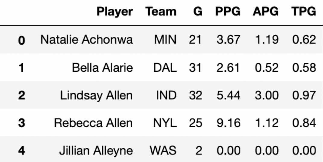
in the WNBA in the 2021 season. The first few rows of
season are shown below.

Each row in season corresponds to a single player. In
this problem, we’ll be working with the 'PPG' column, which
contains the number of points scored per game played.
Suppose we only have access to the DataFrame
small_season, which is a random sample of size
36 from season. We’re interested in learning about
the true mean points per game of all players in season
given just the information in small_season.
To start, we want to bootstrap small_season 10,000 times
and compute the mean of the resample each time. We want to store these
10,000 bootstrapped means in the array boot_means.
Here is a broken implementation of this procedure.
boot_means = np.array([])
for i in np.arange(10000):
    resample = small_season.sample(season.shape[0], replace=False)  # Line 1
    resample_mean = small_season.get('PPG').mean()                  # Line 2
    np.append(boot_means, new_mean)                                 # Line 3
For each of the 3 lines of code above (marked by comments), specify what is incorrect about the line by selecting one or more of the corresponding options below. Or, select “Line _ is correct as-is” if you believe there’s nothing that needs to be changed about the line in order for the above code to run properly.
What is incorrect about Line 1? Select all that apply.
Currently the procedure samples from small_season, when
it should be sampling from season
The sample size is season.shape[0], when it should be
small_season.shape[0]
Sampling is currently being done without replacement, when it should be done with replacement
Line 1 is correct as-is
Answers:
season.shape[0], when it should be
small_season.shape[0]Here, our goal is to bootstrap from small_season. When
bootstrapping, we sample with replacement from our
original sample, with a sample size that’s equal to the original
sample’s size. Here, our original sample is small_season,
so we should be taking samples of size
small_season.shape[0] from it.
Option 1 is incorrect; season has nothing to do with
this problem, as we are bootstrapping from
small_season.
The average score on this problem was 95%.
What is incorrect about Line 2? Select all that apply.
Currently it is taking the mean of the 'PPG' column in
small_season, when it should be taking the mean of the
'PPG' column in season
Currently it is taking the mean of the 'PPG' column in
small_season, when it should be taking the mean of the
'PPG' column in resample
.mean() is not a valid Series method, and should be
replaced with a call to the function np.mean
Line 2 is correct as-is
Answer: Currently it is taking the mean of the
'PPG' column in small_season, when it should
be taking the mean of the 'PPG' column in
resample
The current implementation of Line 2 doesn’t use the
resample at all, when it should. If we were to leave Line 2
as it is, all of the values in boot_means would be
identical (and equal to the mean of the 'PPG' column in
small_season).
Option 1 is incorrect since our bootstrapping procedure is
independent of season. Option 3 is incorrect because
.mean() is a valid Series method.
The average score on this problem was 98%.
What is incorrect about Line 3? Select all that apply.
The result of calling np.append is not being reassigned
to boot_means, so boot_means will be an empty
array after running this procedure
The indentation level of the line is incorrect –
np.append should be outside of the for-loop
(and aligned with for i)
new_mean is not a defined variable name, and should be
replaced with resample_mean
Line 3 is correct as-is
Answers:
np.append is not being reassigned
to boot_means, so boot_means will be an empty
array after running this procedurenew_mean is not a defined variable name, and should be
replaced with resample_meannp.append returns a new array and does not modify the
array it is called on (boot_means, in this case), so Option
1 is a necessary fix. Furthermore, Option 3 is a necessary fix since
new_mean wasn’t defined anywhere.
Option 2 is incorrect; if np.append were outside of the
for-loop, none of the 10,000 resampled means would be saved
in boot_means.
The average score on this problem was 94%.
We construct a 95% confidence interval for the true mean points per game for all players by taking the middle 95% of the bootstrapped sample means.
left_b = np.percentile(boot_means, 2.5)
right_b = np.percentile(boot_means, 97.5)
boot_ci = [left_b, right_b]
Select the most correct statement below.
(left_b + right_b) / 2 is exactly equal to the mean
points per game in season.
(left_b + right_b) / 2 is not necessarily equal to the
mean points per game in season, but is close.
(left_b + right_b) / 2 is exactly equal to the mean
points per game in small_season.
(left_b + right_b) / 2 is not necessarily equal to the
mean points per game in small_season, but is close.
(left_b _+ right_b) / 2 is not close to either the mean
points per game in season or the mean points per game in
small_season.
Answer: (left_b + right_b) / 2 is not
necessarily equal to the mean points per game in
small_season, but is close.
Normal-based confidence intervals are of the form [\text{mean} - \text{something}, \text{mean} + \text{something}]. In such confidence intervals, it is the case that the average of the left and right endpoints is exactly the mean of the distribution used to compute the interval.
However, the confidence interval we’ve created is not normal-based, rather it is bootstrap-based! As such, we can’t say that anything is exactly true; this rules out Options 1 and 3.
Our 95% confidence interval was created by taking the middle 95% of
bootstrapped sample means. The distribution of bootstrapped sample means
is roughly normal, and the normal distribution is
symmetric (the mean and median are both equal, and represent the
“center” of the distribution). This means that the middle of our 95%
confidence interval should be roughly equal to the mean of the
distribution of bootstrapped sample means. This implies that Option 4 is
correct; the difference between Options 2 and 4 is that Option 4 uses
small_season, which is the sample we bootstrapped from,
while Option 2 uses season, which was not accessed at all
in our bootstrapping procedure.
The average score on this problem was 62%.
Rank these three students in ascending order of their exam performance relative to their classmates.
Hector, Clara, Vivek
Vivek, Hector, Clara
Clara, Hector, Vivek
Vivek, Clara, Hector
Answer: Vivek, Hector, Clara
To compare Vivek, Hector, and Clara’s relative performance we want to compare their Z scores to handle standardization. For Vivek, his Z score is (83-75) / 6 = 4/3. For Hector, his score is (77-70) / 5 = 7/5. For Clara, her score is (80-75) / 3 = 5/3. Ranking these, 5/3 > 7/5 > 4/3 which yields the result of Vivek, Hector, Clara.
The average score on this problem was 76%.
The data visualization below shows all Olympic gold medals for women’s gymnastics, broken down by the age of the gymnast.

Based on this data, rank the following three quantities in ascending order: the median age at which gold medals are earned, the mean age at which gold medals are earned, the standard deviation of the age at which gold medals are earned.
mean, median, SD
median, mean, SD
SD, mean, median
SD, median, mean
Answer: SD, median, mean
The standard deviation will clearly be the smallest of the three
values as most of the data is encompassed between the range of
[14-26]. Intuitively, the standard deviation will have to
be about a third of this range which is around 4 (though this is not the
exact standard deviation, but is clearly much less than the mean and
median with values closer to 19-25). Comparing the median and mean, it
is important to visualize that this distribution is skewed right. When
the data is skewed right it pulls the mean towards a higher value (as
the higher values naturally make the average higher). Therefore, we know
that the mean will be greater than the median and the ranking is SD,
median, mean.
The average score on this problem was 72%.
Among all Costco members in San Diego, the average monthly spending in October 2023 was $350 with a standard deviation of $40.
The amount Ciro spent at Costco in October 2023 was -1.5 in standard units. What is this amount in dollars? Give your answer as an integer.
Answer: 290
The average score on this problem was 93%.
What is the minimum possible percentage of San Diego members that spent between $250 and $450 in October 2023?
16%
22%
36%
60%
78%
84%
Answer: 84%
The average score on this problem was 61%.
Now, suppose we’re given that the distribution of monthly spending in October 2023 for all San Diego members is roughly normal. Given this fact, fill in the blanks:
What are m and n? Give your answers as integers rounded to the nearest multiple of 10.
Answer: m: 270, n: 430
The average score on this problem was 81%.
Suppose we have access to a simple random sample of all US Costco
members of size 145. Our sample is stored in a
DataFrame named us_sample, in which the
"Spend" column contains the October 2023 spending of each
sampled member in dollars.
Fill in the blanks below so that us_left and
us_right are the left and right endpoints of a
46% confidence interval for the average October 2023
spending of all US members.
costco_means = np.array([])
for i in np.arange(5000):
    resampled_spends = __(x)__
    costco_means = np.append(costco_means, resampled_spends.mean())
us_left = np.percentile(costco_means, __(y)__)
us_right = np.percentile(costco_means, __(z)__)
Which of the following could go in blank (x)? Select all that apply.
us_sample.sample(145, replace=True).get("Spend")
us_sample.sample(145, replace=False).get("Spend")
np.random.choice(us_sample.get("Spend"), 145)
np.random.choice(us_sample.get("Spend"), 145, replace=True)
np.random.choice(us_sample.get("Spend"), 145, replace=False)
None of the above.
What goes in blanks (y) and (z)? Give your answers as integers.
Answer:
x:
us_sample.sample(145, replace=True).get("Spend")np.random.choice(us_sample.get("Spend"), 145)np.random.choice(us_sample.get("Spend"), 145, replace=True)y: 27z: 73
The average score on this problem was 79%.
True or False: 46% of all US members in
us_sample spent between us_left and
us_right in October 2023.
True
False
Answer: False
The average score on this problem was 85%.
True or False: If we repeat the code from part (b) 200 times, each time bootstrapping from a new random sample of 145 members drawn from all US members, then about 92 of the intervals we create will contain the average October 2023 spending of all US members.
True
False
Answer: True
The average score on this problem was 51%.
True or False: If we repeat the code from part (b) 200 times, each
time bootstrapping from us_sample, then about
92 of the intervals we create will contain the average
October 2023 spending of all US members.
True
False
Answer: False
The average score on this problem was 30%.
Researchers from the San Diego Zoo, located within Balboa Park, collected physical measurements of several species of penguins in a region of Antarctica.
One piece of information they tracked for each of 330 penguins was its mass in grams. The average penguin mass is 4200 grams, and the standard deviation is 840 grams.
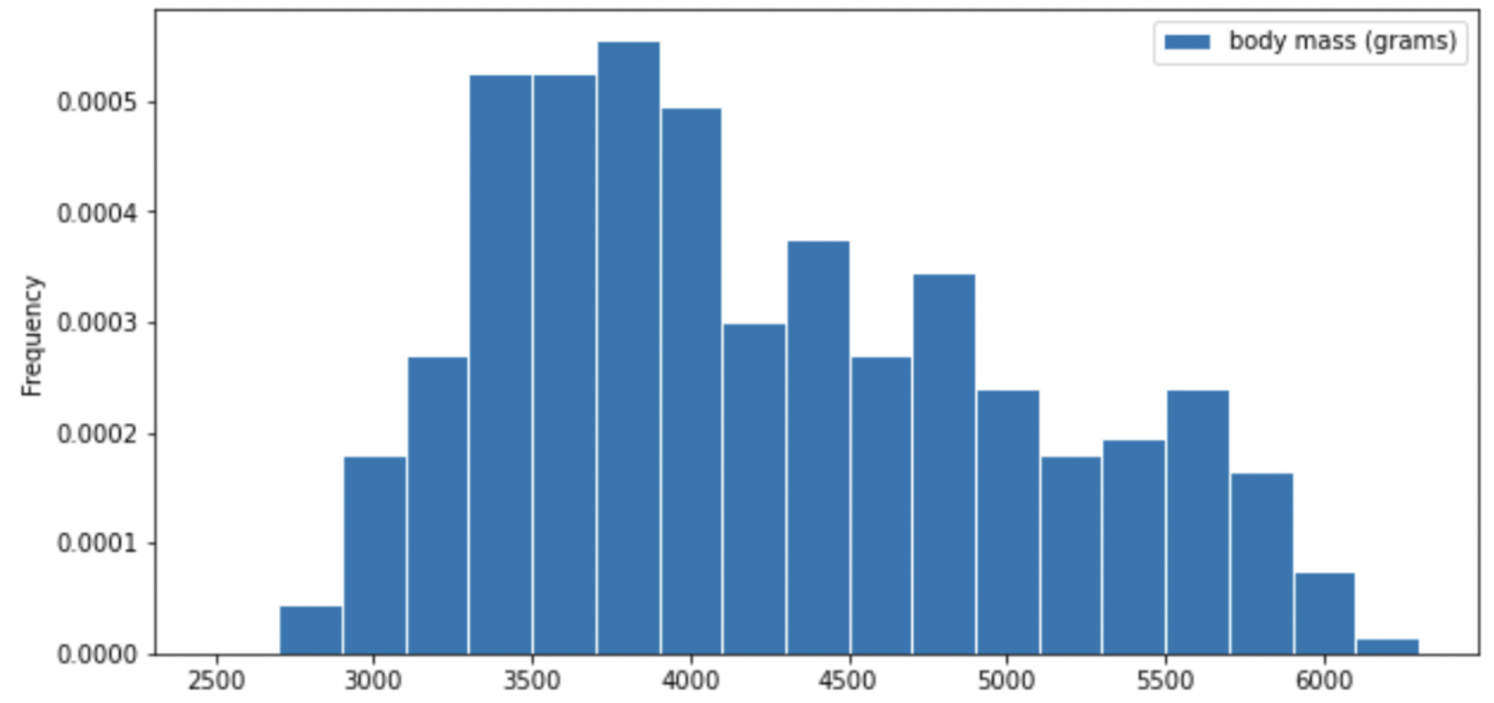
Consider the histogram of mass below.

Select the true statement below.
The median mass of penguins is larger than the average mass of penguins
The median mass of penguins is roughly equal to the average mass of penguins (within 50 grams)
The median mass of penguins is less than the average mass of penguins
It is impossible to determine the relationship between the median and average mass of penguins just by looking at the above histogram
Answer: The median mass of penguins is less than the average mass of penguins
This is a distribution that is skewed to the right, so mean is greater than median.
The average score on this problem was 87%.
For your convenience, we show the histogram of mass again below.

Recall, there are 330 penguins in our dataset. Their average mass is 4200 grams, and the standard deviation of mass is 840 grams.
Per Chebyshev’s inequality, at least what percentage of penguins have a mass between 3276 grams and 5124 grams? Input your answer as a percentage between 0 and 100, without the % symbol. Round to three decimal places.
Answer: 17.355
Recall, Chebyshev’s inequality states that No matter what the shape of the distribution is, the proportion of values in the range “average ± z SDs” is at least 1 - \frac{1}{z^2}.
To approach the problem, we’ll start by converting 3276 grams and 5124 grams to standard units. Doing so yields \frac{3276 - 4200}{840} = -1.1, similarly, \frac{5124 - 4200}{840} = 1.1. This means that 3276 is 1.1 standard deviations below the mean, and 5124 is 1.1 standard deviations above the mean. Thus, we are calculating the proportion of values in the range “average ± 1.1 SDs”.
When z = 1.1, we have 1 - \frac{1}{z^2} = 1 - \frac{1}{1.1^2} \approx 0.173553719, which as a percentage rounded to three decimal places is 17.355\%.
The average score on this problem was 76%.
Per Chebyshev’s inequality, at least what percentage of penguins have a mass between 1680 grams and 5880 grams?
50%
55.5%
65.25%
68%
75%
88.8%
95%
Answer: 75%
Recall: proportion with z SDs of the mean
| Percent in Range | All Distributions (via Chebyshev’s Inequality) | Normal Distributions |
|---|---|---|
| \text{average} \pm 1 \ \text{SD} | \geq 0\% | \approx 68\% |
| \text{average} \pm 2\text{SDs} | \geq 75\% | \approx 95\% |
| \text{average} \pm 3\text{SDs} | \geq 88\% | \approx 99.73\% |
To approach the problem, we’ll start by converting 3276 grams and 5124 grams to standard units. Doing so yields \frac{1680 - 4200}{840} = -3, similarly, \frac{5880 - 4200}{840} = 2. This means that 1680 is 3 standard deviations below the mean, and 5880 is 2 standard deviations above the mean.
Proportion of values in [-3 SUs, 2 SUs] >= Proportion of values in [-2 SUs, 2 SUs] >= 75% (Since we cannot assume that the distribution is normal, we look at the All Distributions (via Chebyshev’s Inequality) column for proportion).
Thus, at least 75% of the penguins have a mass between 1680 grams and 5880 grams.
The average score on this problem was 72%.
The distribution of mass in grams is not roughly normal. Is the distribution of mass in standard units roughly normal?
Yes
No
Impossible to tell
Answer: No
The shape of the distribution does not change since we are scaling the x values for all data.
The average score on this problem was 60%.
Suppose boot_means is an array of the resampled means.
Fill in the blanks below so that [left, right] is a 68%
confidence interval for the true mean mass of penguins.
left = np.percentile(boot_means, __(a)__)
right = np.percentile(boot_means, __(b)__)
[left, right]
What goes in blank (a)? What goes in blank (b)?
Answer: (a) 16 (b) 84
Recall, np.percentile(array, p) computes the
pth percentile of the numbers in array. To
compute the 68% CI, we need to know the percentile of left tail and
right tail.
left percentile = (1-0.68)/2 = (0.32)/2 = 0.16 so we have 16th percentile
right percentile = 1-((1-0.68)/2) = 1-((0.32)/2) = 1-0.16 = 0.84 so we have 84th percentile
The average score on this problem was 94%.
Which of the following is a correct interpretation of this confidence interval? Select all that apply.
There is an approximately 68% chance that mean weight of all penguins in Antarctica falls within the bounds of this confidence interval.
Approximately 68% of penguin weights in our sample fall within the bounds of this confidence interval.
Approximately 68% of penguin weights in the population fall within the bounds of this interval.
If we created many confidence intervals using the same method, approximately 68% of them would contain the mean weight of all penguins in Antarctica.
None of the above
Answer: Option 4 (If we created many confidence intervals using the same method, approximately 68% of them would contain the mean weight of all penguins in Antarctica.)
Recall, what a k% confidence level states is that approximately k% of the time, the intervals you create through this process will contain the true population parameter.
In this question, our population parameter is the mean weight of all penguins in Antarctica. So 86% of the time, the intervals you create through this process will contain the mean weight of all penguins in Antarctica. This is the same as Option 4. However, it will be false if we state it in the reverse order (Option 1) since our population parameter is already fixed.
The average score on this problem was 81%.