← return to practice.dsc10.com
Welcome! The problems shown below should be worked on on
paper, since the quizzes and exams you take in this course will
also be on paper. You do not need to submit your solutions anywhere.
We encourage you to complete this worksheet in groups during an
extra practice session on Friday, February 23th. Solutions will be
posted after all sessions have finished. This problem set is not
designed to take any particular amount of time - focus on understanding
concepts, not on getting through all the questions.
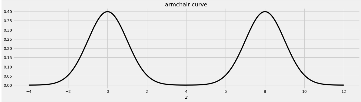
An IKEA chair designer is experimenting with some new ideas for armchair designs. She has the idea of making the arm rests shaped like bell curves, or normal distributions. A cross-section of the armchair design is shown below.
This was created by taking the portion of the standard normal distribution from z=-4 to z=4 and adjoining two copies of it, one centered at z=0 and the other centered at z=8. Let’s call this shape the armchair curve.
Since the area under the standard normal curve from z=-4 to z=4 is approximately 1, the total area under the armchair curve is approximately 2.
Complete the implementation of the two functions below:
area_left_of(z) should return the area under the
armchair curve to the left of z, assuming
-4 <= z <= 12, andarea_between(x, y) should return the area under the
armchair curve between x and y, assuming
-4 <= x <= y <= 12.import scipy
def area_left_of(z):
'''Returns the area under the armchair curve to the left of z.
Assume -4 <= z <= 12'''
if ___(a)___:
return ___(b)___
return scipy.stats.norm.cdf(z)
def area_between(x, y):
'''Returns the area under the armchair curve between x and y.
Assume -4 <= x <= y <= 12.'''
return ___(c)___What goes in blank (a)?
Answer: z>4 or
z>=4
The body of the function contains an if statement
followed by a return statement, which executes only when
the if condition is false. In that case, the function
returns scipy.stats.norm.cdf(z), which is the area under
the standard normal curve to the left of z. When
z is in the left half of the armchair curve, the area under
the armchair curve to the left of z is the area under the
standard normal curve to the left of z because the left
half of the armchair curve is a standard normal curve, centered at 0. So
we want to execute the return statement in that case, but
not if z is in the right half of the armchair curve, since
in that case the area to the left of z under the armchair
curve should be more than 1, and scipy.stats.norm.cdf(z)
can never exceed 1. This means the if condition needs to
correspond to z being in the right half of the armchair
curve, which corresponds to z>4 or z>=4,
either of which is a correct solution.
The average score on this problem was 72%.
What goes in blank (b)?
Answer:
1+scipy.stats.norm.cdf(z-8)
This blank should contain the value we want to return when
z is in the right half of the armchair curve. In this case,
the area under the armchair curve to the left of z is the
sum of two areas:
z.Since the right half of the armchair curve is just a standard normal
curve that’s been shifted to the right by 8 units, the area under that
normal curve to the left of z is the same as the area to
the left of z-8 on the standard normal curve that’s
centered at 0. Adding the portion from the left half and the right half
of the armchair curve gives
1+scipy.stats.norm.cdf(z-8).
For example, if we want to find the area under the armchair curve to the left of 9, we need to total the yellow and blue areas in the image below.
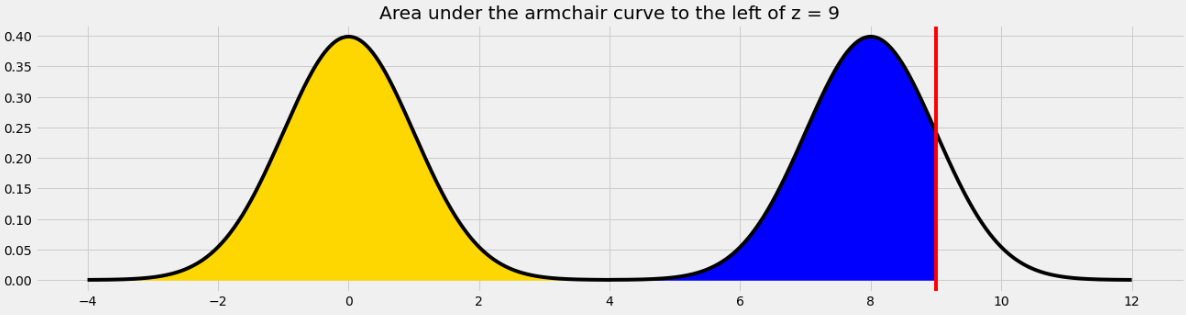
The yellow area is 1 and the blue area is the same as the area under the standard normal curve (or the left half of the armchair curve) to the left of 1 because 1 is the point on the left half of the armchair curve that corresponds to 9 on the right half. In general, we need to subtract 8 from a value on the right half to get the corresponding value on the left half.
The average score on this problem was 54%.
What goes in blank (c)?
Answer:
area_left_of(y) - area_left_of(x)
In general, we can find the area under any curve between
x and y by taking the area under the curve to
the left of y and subtracting the area under the curve to
the left of x. Since we have a function to find the area to
the left of any given point in the armchair curve, we just need to call
that function twice with the appropriate inputs and subtract the
result.
The average score on this problem was 60%.
Oren has a random sample of 200 dog prices in an array called
oren. He has also bootstrapped his sample 1,000 times and
stored the mean of each resample in an array called
boots.
In this question, assume that the following code has run:
a = np.mean(oren)
b = np.std(oren)
c = len(oren)What expression best estimates the population’s standard deviation?
b
b / c
b / np.sqrt(c)
b * np.sqrt(c)
Answer: b
The function np.std directly calculated the standard
deviation of array oren. Even though oren is
sample of the population, its standard deviation is still a pretty good
estimate for the standard deviation of the population because it is a
random sample. The other options don’t really make sense in this
context.
The average score on this problem was 57%.
Which expression best estimates the mean of boots?
0
a
(oren - a).mean()
(oren - a) / b
Answer: a
Note that a is equal to the mean of oren,
which is a pretty good estimator of the mean of the overall population
as well as the mean of the distribution of sample means. The other
options don’t really make sense in this context.
The average score on this problem was 89%.
What expression best estimates the standard deviation of
boots?
b
b / c
b / np.sqrt(c)
(a -b) / np.sqrt(c)
Answer: b / np.sqrt(c)
Note that we can use the Central Limit Theorem for this problem which
states that the standard deviation (SD) of the distribution of sample
means is equal to (population SD) / np.sqrt(sample size).
Since the SD of the sample is also the SD of the population in this
case, we can plug our variables in to see that
b / np.sqrt(c) is the answer.
The average score on this problem was 91%.
What is the dog price of $560 in standard units?
(560 - a) / b
(560 - a) / (b / np.sqrt(c))
(a - 560) / (b / np.sqrt(c))}
abs(560 - a) / b
abs(560 - a) / (b / np.sqrt(c))
Answer: (560 - a) / b
To convert a value to standard units, we take the value, subtract the
mean from it, and divide by SD. In this case that is
(560 - a) / b, because a is the mean of our
dog prices sample array and b is the SD of the dog prices
sample array.
The average score on this problem was 80%.
The distribution of boots is normal because of the
Central Limit Theorem.
True
False
Answer: True
True. The central limit theorem states that if you have a population and you take a sufficiently large number of random samples from the population, then the distribution of the sample means will be approximately normally distributed.
The average score on this problem was 91%.
If Oren’s sample was 400 dogs instead of 200, the standard deviation
of boots will…
Increase by a factor of 2
Increase by a factor of \sqrt{2}
Decrease by a factor of 2
Decrease by a factor of \sqrt{2}
None of the above
Answer: Decrease by a factor of \sqrt{2}
Recall that the central limit theorem states that the STD of the
sample distribution is equal to
(population STD) / np.sqrt(sample size). So if we increase
the sample size by a factor of 2, the STD of the sample distribution
will decrease by a factor of \sqrt{2}.
The average score on this problem was 80%.
If Oren took 4000 bootstrap resamples instead of 1000, the standard
deviation of boots will…
Increase by a factor of 4
Increase by a factor of 2
Decrease by a factor of 2
Decrease by a factor of 4
None of the above
Answer: None of the above
Again, from our formula given by the central limit theorem, the
sample STD doesn’t depend on the number of bootstrap resamples so long
as it’s “sufficiently large”. Thus increasing our bootstrap sample from
1000 to 4000 will have no effect on the std of boots
The average score on this problem was 74%.
Write one line of code that evaluates to the right endpoint of a 92% CLT-Based confidence interval for the mean dog price. The following expressions may help:
stats.norm.cdf(1.75) # => 0.96
stats.norm.cdf(1.4) # => 0.92Answer: a + 1.75 * b / np.sqrt(c)
Recall that a 92% confidence interval means an interval that consists
of the middle 92% of the distribution. In other words, we want to “chop”
off 4% from either end of the ditribution. Thus to get the right
endpoint, we want the value corresponding to the 96th percentile in the
mean dog price distribution, or
mean + 1.75 * (SD of population / np.sqrt(sample size) or
a + 1.75 * b / np.sqrt(c) (we divide by
np.sqrt(c) due to the central limit theorem). Note that the
second line of information that was given
stats.norm.cdf(1.4) is irrelavant to this particular
problem.
The average score on this problem was 48%.
From a population with mean 500 and standard deviation 50, you collect a sample of size 100. The sample has mean 400 and standard deviation 40. You bootstrap this sample 10,000 times, collecting 10,000 resample means.
Which of the following is the most accurate description of the mean of the distribution of the 10,000 bootstrapped means?
The mean will be exactly equal to 400.
The mean will be exactly equal to 500.
The mean will be approximately equal to 400.
The mean will be approximately equal to 500.
Answer: The mean will be approximately equal to 400.
The distribution of bootstrapped means’ mean will be approximately 400 since that is the mean of the sample and bootstrapping is taking many samples of the original sample. The mean will not be exactly 400 do to some randomness though it will be very close.
The average score on this problem was 54%.
Which of the following is closest to the standard deviation of the distribution of the 10,000 bootstrapped means?
400
40
4
0.4
Answer: 4
To find the standard deviation of the distribution, we can take the sample standard deviation S divided by the square root of the sample size. From plugging in, we get 40 / 10 = 4.
The average score on this problem was 51%.
We collect data on the play times of 100 games of Chutes and Ladders (sometimes known as Snakes and Ladders).
We use our collected data to construct a 95% CLT-based confidence interval for the average play time of a game of Chutes and Ladders. This 95% confidence interval is [26.47, 28.47]. For the 100 games for which we collected data, what is the mean and standard deviation of the play times?
Answer: mean = 27.47 and SD = 5
One of the key properties of the normal distribution is that about 95% of values lie within 2 standard deviations of the mean. The Central Limit Theorem states that the distribution of the sample mean is roughly normal, which means that to create this CLT-based 95% confidence interval, we used the 2 standard deviations rule.
What we’re given, then, is the following:
\begin{align*} \text{Sample Mean} + 2 \cdot \text{SD of Distribution of Possible Sample Means} &= 28.47 \\ \text{Sample Mean} - 2 \cdot \text{SD of Distribution of Possible Sample Means} &= 26.47 \end{align*}
The sample mean is halfway between 26.47 and 28.47, which is 27.47. Substituting this into the first equation gives us
\begin{align*}27.47 + 2 \cdot \text{SD of Distribution of Possible Sample Means} &= 28.47\\2 \cdot \text{SD of Distribution of Possible Sample Means} &= 1 \\ \text{Distribution of Possible Sample Means} &= 0.5\end{align*}
It can be tempting to conclude that the sample standard deviation is 0.5, but it’s not – the SD of the sample mean’s distribution is 0.5. Remember, the SD of the sample mean’s distribution is given by the square root law:
\text{SD of Distribution of Possible Sample Means} = \frac{\text{Population SD}}{\sqrt{\text{Sample Size}}} \approx \frac{\text{Sample SD}}{\sqrt{\text{Sample Size}}}
We don’t know the population SD, so we’ve used the sample SD as an estimate. As such, we have that
\text{SD of Distribution of Possible Sample Means} = 0.5 = \frac{\text{Sample SD}}{\sqrt{\text{Sample Size}}} = \frac{\text{Sample SD}}{\sqrt{100}}
So, \text{Sample SD} = 0.5 \cdot \sqrt{100} = 0.5 \cdot 10 = 5.
The average score on this problem was 64%.
Does the CLT say that the distribution of play times of the 100 games is roughly normal?
Yes
No
Answer: No
The Central Limit Theorem states that the distribution of the sample mean or the sample sum is roughly normal. The distribution of play times is a sample of size 100 drawn from the population of play times; the Central Limit Theorem doesn’t say anything about a population or any one sample.
The average score on this problem was 45%.
It’s your first time playing a new game called Brunch Menu. The deck contains 96 cards, and each player will be dealt a hand of 9 cards. The goal of the game is to avoid having certain cards, called Rotten Egg cards, which come with a penalty at the end of the game. But you’re not sure how many of the 96 cards in the game are Rotten Egg cards. So you decide to use the Central Limit Theorem to estimate the proportion of Rotten Egg cards in the deck based on the 9 random cards you are dealt in your hand.
You are dealt 3 Rotten Egg cards in your hand of 9 cards. You then construct a CLT-based 95% confidence interval for the proportion of Rotten Egg cards in the deck based on this sample. Approximately, how wide is your confidence interval?
Choose the closest answer, and use the following facts:
The standard deviation of a collection of 0s and 1s is \sqrt{(\text{Prop. of 0s}) \cdot (\text{Prop of 1s})}.
\sqrt{18} is about \frac{17}{4}.
\frac{17}{9}
\frac{17}{27}
\frac{17}{81}
\frac{17}{96}
Answer: \frac{17}{27}
A Central Limit Theorem-based 95% confidence interval for a population proportion is given by the following:
\left[ \text{Sample Proportion} - 2 \cdot \frac{\text{Sample SD}}{\sqrt{\text{Sample Size}}}, \text{Sample Proportion} + 2 \cdot \frac{\text{Sample SD}}{\sqrt{\text{Sample Size}}} \right]
Note that this interval uses the fact that (about) 95% of values in a normal distribution are within 2 standard deviations of the mean. It’s key to divide by \sqrt{\text{Sample Size}} when computing the standard deviation because the distribution that is roughly normal is the distribution of the sample mean (and hence, sample proportion), not the distribution of the sample itself.
The width of the above interval – that is, the right endpoint minus the left endpoint – is
\text{width} = 4 \cdot \frac{\text{Sample SD}}{\sqrt{\text{Sample Size}}}
From the provided hint, we have that
\text{Sample SD} = \sqrt{(\text{Prop. of 0s}) \cdot (\text{Prop of 1s})} = \sqrt{\frac{3}{9} \cdot \frac{6}{9}} = \frac{\sqrt{18}}{9}
Then, since we know that the sample size is 9 and that \sqrt{18} is about \frac{17}{4}, we have
\text{width} = 4 \cdot \frac{\text{Sample SD}}{\sqrt{\text{Sample Size}}} = 4 \cdot \frac{\frac{\sqrt{18}}{9}}{\sqrt{9}} = 4 \cdot \frac{\sqrt{18}}{9 \cdot 3} = 4 \cdot \frac{\frac{17}{4}}{27} = \frac{17}{27}
The average score on this problem was 51%.
Which of the following are limitations of trying to use the Central Limit Theorem for this particular application? Select all that apply.
The CLT is for large random samples, and our sample was not very large.
The CLT is for random samples drawn with replacement, and our sample was drawn without replacement.
The CLT is for normally distributed data, and our data may not have been normally distributed.
The CLT is for sample means and sums, not sample proportions.
Answer: Options 1 and 2
Option 1: We use Central Limit Theorem (CLT) for large random samples, and a sample of 9 is considered to be very small. This makes it difficult to use CLT for this problem.
Option 2: Recall CLT happens when our sample is drawn with replacement. When we are handed nine cards we are never replacing cards back into our deck, which means that we are sampling without replacement.
Option 3: This is wrong because CLT states that a large sample is approximately a normal distribution even if the data itself is not normally distributed. This means it doesn’t matter if our data had not been normally distributed if we had a large enough sample we could use CLT.
Option 4: This is wrong because CLT does apply to the sample proportion distribution. Recall that proportions can be treated like means.
The average score on this problem was 77%.
Suppose you draw a sample of size 100 from a population with mean 50 and standard deviation 15. What is the probability that your sample has a mean between 50 and 53? Input the probability below, as a number between 0 and 1, rounded to two decimal places.
Answer: 0.48
This problem is testing our understanding of the Central Limit Theorem and normal distributions. Recall, the Central Limit Theorem tells us that the distribution of the sample mean is roughly normal, with the following characteristics:
\begin{align*} \text{Mean of Distribution of Possible Sample Means} &= \text{Population Mean} = 50 \\ \text{SD of Distribution of Possible Sample Means} &= \frac{\text{Population SD}}{\sqrt{\text{Sample Size}}} = \frac{15}{\sqrt{100}} = 1.5 \end{align*}
Given this information, it may be easier to express the problem as “We draw a value from a normal distribution with mean 50 and SD 1.5. What is the probability that the value is between 50 and 53?” Note that this probability is equal to the proportion of values between 50 and 53 in a normal distribution whose mean is 50 and 1.5 (since probabilities can be thought of as proportions).
In class, we typically worked with the standard normal distribution, in which the mean was 0, the SD was 1, and the x-axis represented values in standard units. Let’s convert the quantities of interest in this problem to standard units, keeping in mind that the mean and SD we’re using now are the mean and SD of the distribution of possible sample means, not of the population.
Now, our problem boils down to finding the proportion of values in a standard normal distribution that are between 0 and 2, or the proportion of values in a normal distribution that are in the interval [\text{mean}, \text{mean} + 2 \text{ SDs}].
From class, we know that in a normal distribution, roughly 95% of values are within 2 standard deviations of the mean, i.e. the proportion of values in the interval [\text{mean} - 2 \text{ SDs}, \text{mean} + 2 \text{ SDs}] is 0.95.
Since the normal distribution is symmetric about the mean, half of the values in this interval are to the right of the mean, and half are to the left. This means that the proportion of values in the interval [\text{mean}, \text{mean} + 2 \text{ SDs}] is \frac{0.95}{2} = 0.475, which rounds to 0.48, and thus the desired result is 0.48.
The average score on this problem was 48%.
The DataFrame apps contains application data for a
random sample of 1,000 applicants for a particular credit card from the
1990s. The "age" column contains the applicants’ ages, in
years, to the nearest twelfth of a year.
The credit card company that owns the data in apps,
BruinCard, has decided not to give us access to the entire
apps DataFrame, but instead just a random sample of 100
rows of apps called hundred_apps.
We are interested in estimating the mean age of all applicants in
apps given only the data in hundred_apps. The
ages in hundred_apps have a mean of 35 and a standard
deviation of 10.
Give the endpoints of the CLT-based 95% confidence interval for the
mean age of all applicants in apps, based on the data in
hundred_apps.
Answer: Left endpoint = 33, Right endpoint = 37
According to the Central Limit Theorem, the standard deviation of the distribution of the sample mean is \frac{\text{sample SD}}{\sqrt{\text{sample size}}} = \frac{10}{\sqrt{100}} = 1. Then using the fact that the distribution of the sample mean is roughly normal, since 95% of the area of a normal curve falls within two standard deviations of the mean, we can find the endpoints of the 95% CLT-based confidence interval as 35 - 2 = 33 and 35 + 2 = 37.
We can think of this as using the formula below: \left[\text{sample mean} - 2\cdot \frac{\text{sample SD}}{\sqrt{\text{sample size}}}, \: \text{sample mean} + 2\cdot \frac{\text{sample SD}}{\sqrt{\text{sample size}}} \right]. Plugging in the appropriate quantities yields [35 - 2\cdot\frac{10}{\sqrt{100}}, 35 - 2\cdot\frac{10}{\sqrt{100}}] = [33, 37].
The average score on this problem was 67%.
BruinCard reinstates our access to apps so that we can
now easily extract information about the ages of all applicants. We
determine that, just like in hundred_apps, the ages in
apps have a mean of 35 and a standard deviation of 10. This
raises the question of how other samples of 100 rows of
apps would have turned out, so we compute 10,000 sample means as follows.
    sample_means = np.array([])
    for i in np.arange(10000):
        sample_mean = apps.sample(100, replace=True).get("age").mean()
        sample_means = np.append(sample_means, sample_mean)
Which of the following three visualizations best depict the
distribution of sample_means?
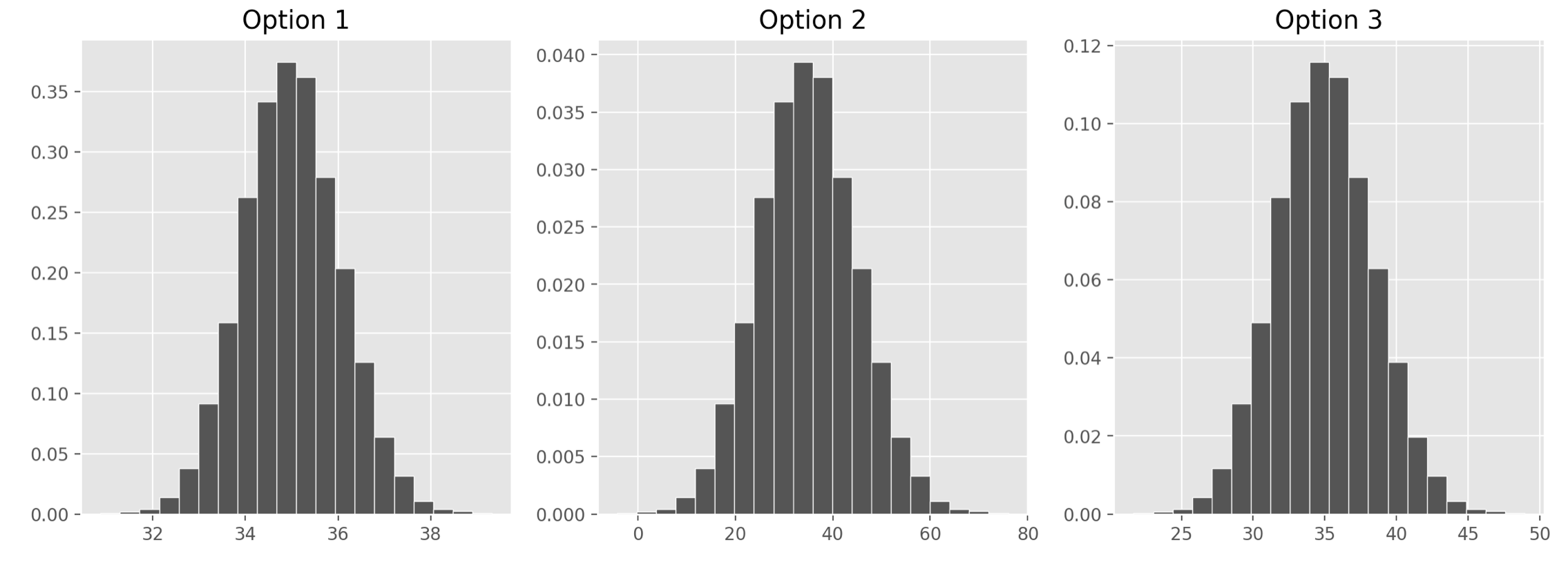
Answer: Option 1
As we found in the previous part, the distribution of the sample mean should have a standard deviation of 1. We also know it should be centered at the mean of our sample, at 35, but since all the options are centered here, that’s not too helpful. Only Option 1, however, has a standard deviation of 1. Remember, we can approximate the standard deviation of a normal curve as the distance between the mean and either of the inflection points. Only Option 1 looks like it has inflection points at 34 and 36, a distance of 1 from the mean of 35.
If you chose Option 2, you probably confused the standard deviation of our original sample, 10, with the standard deviation of the distribution of the sample mean, which comes from dividing that value by the square root of the sample size.
The average score on this problem was 57%.
Which of the following statements are guaranteed to be true? Select all that apply.
We used bootstrapping to compute sample_means.
The ages of credit card applicants are roughly normally distributed.
A CLT-based 90% confidence interval for the mean age of credit card applicants, based on the data in hundred apps, would be narrower than the interval you gave in part (a).
The expression np.percentile(sample_means, 2.5)
evaluates to the left endpoint of the interval you gave in part (a).
If we used the data in hundred_apps to create 1,000
CLT-based 95% confidence intervals for the mean age of applicants in
apps, approximately 950 of them would contain the true mean
age of applicants in apps.
None of the above.
Answer: A CLT-based 90% confidence interval for the
mean age of credit card applicants, based on the data in
hundred_apps, would be narrower than the interval you gave
in part (a).
Let’s analyze each of the options:
Option 1: We are not using bootstrapping to compute sample means
since we are sampling from the apps DataFrame, which is our
population here. If we were bootstrapping, we’d need to sample from our
first sample, which is hundred_apps.
Option 2: We can’t be sure what the distribution of the ages of
credit card applicants are. The Central Limit Theorem says that the
distribution of sample_means is roughly normally
distributed, but we know nothing about the population
distribution.
Option 3: The CLT-based 95% confidence interval that we calculated in part (a) was computed as follows: \left[\text{sample mean} - 2\cdot \frac{\text{sample SD}}{\sqrt{\text{sample size}}}, \text{sample mean} + 2\cdot \frac{\text{sample SD}}{\sqrt{\text{sample size}}} \right] A CLT-based 90% confidence interval would be computed as \left[\text{sample mean} - z\cdot \frac{\text{sample SD}}{\sqrt{\text{sample size}}}, \text{sample mean} + z\cdot \frac{\text{sample SD}}{\sqrt{\text{sample size}}} \right] for some value of z less than 2. We know that 95% of the area of a normal curve is within two standard deviations of the mean, so to only pick up 90% of the area, we’d have to go slightly less than 2 standard deviations away. This means the 90% confidence interval will be narrower than the 95% confidence interval.
Option 4: The left endpoint of the interval from part (a) was
calculated using the Central Limit Theorem, whereas using
np.percentile(sample_means, 2.5) is calculated empirically,
using the data in sample_means. Empirically calculating a
confidence interval doesn’t necessarily always give the exact same
endpoints as using the Central Limit Theorem, but it should give you
values close to those endpoints. These values are likely very similar
but they are not guaranteed to be the same. One way to see this is that
if we ran the code to generate sample_means again, we’d
probably get a different value for
np.percentile(sample_means, 2.5).
Option 5: The key observation is that if we used the data in
hundred_apps to create 1,000 CLT-based 95% confidence
intervals for the mean age of applicants in apps, all of
these intervals would be exactly the same. Given a sample, there is only
one CLT-based 95% confidence interval associated with it. In our case,
given the sample hundred_apps, the one and only CLT-based
95% confidence interval based on this sample is the one we found in part
(a). Therefore if we generated 1,000 of these intervals, either they
would all contain the parameter or none of them would. In order for a
statement like the one here to be true, we would need to collect 1,000
different samples, and calculate a confidence interval from each
one.
The average score on this problem was 49%.
You want to estimate the proportion of DSC majors who have a Netflix subscription. To do so, you will survey a random sample of DSC majors and ask them whether they have a Netflix subscription. You will then create a 95% confidence interval for the proportion of “yes" answers in the population, based on the responses in your sample. You decide that your confidence interval should have a width of at most 0.10.
In order for your confidence interval to have a width of at most 0.10, the standard deviation of the distribution of the sample proportion must be at most T. What is T? Give your answer as an exact decimal.
Answer: 0.025
The average score on this problem was 46%.
Using the fact that the standard deviation of any dataset of 0s and 1s is no more than 0.5, calculate the minimum number of people you would need to survey so that the width of your confidence interval is at most 0.10. Give your answer as an integer.
Answer: 400
The average score on this problem was 81%.