← return to practice.dsc10.com
Instructor(s): Janine Tiefenbruck
This exam was administered in-person. The exam was closed-notes, except students were provided a copy of the DSC 10 Reference Sheet. No calculators were allowed. Students had 3 hours to take this exam.
Note (groupby / pandas 2.0): Pandas 2.0+ no longer
silently drops columns that can’t be aggregated after a
groupby, so code written for older pandas may behave
differently or raise errors. In these practice materials we use
.get() to select the column(s) we want after
.groupby(...).mean() (or other aggregations) so that our
solutions run on current pandas. On real exams you will not be penalized
for omitting .get() when the old behavior would have
produced the same answer.
Welcome to
![]() !
!
IKEA is a Swedish furniture company that designs and sells ready-to-assemble furniture and other home furnishings. IKEA has locations worldwide, including one in San Diego. IKEA is known for its cheap prices, modern designs, huge showrooms, and wordless instruction manuals. They also sell really good Swedish meatballs in their cafe!

This exam is all about IKEA. Here are the DataFrames you’ll be working with:
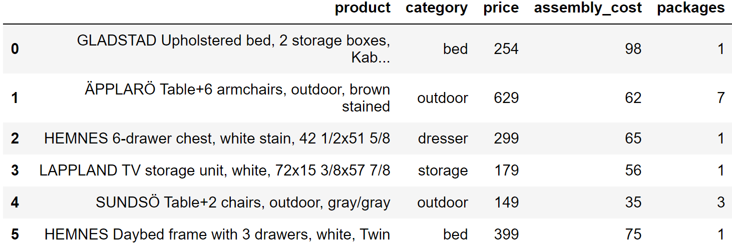
ikeaThe ikea DataFrame has a row for each ready-to-assemble
IKEA furniture product. The columns are:
'product' (str): the name of the product,
which includes the product line as the first word, followed by a
description of the product'category' (str): a categorical
description of the type of product'price' (int): the current price of the
product, in dollars'assembly_cost' (int): the additional cost
to have the product assembled, in dollars'packages' (int): the number of packages
in which the product is boxedThe first few rows of ikea are shown below, though
ikea has many more rows than pictured.
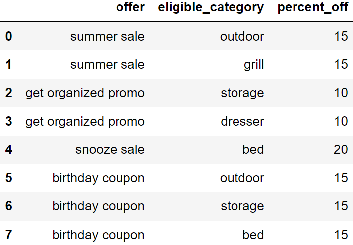
offersIKEA sometimes runs certain special offers, including coupons, sales,
and promotions. For each offer currently available, the DataFrame
offers has a separate row for each category of products to
which the offer can be applied. The columns are:
'offer' (str): the name of the offer'category' (str): the category to which
the offer applies'percent_off' (int): the percent discount
when applying this offer to this categoryThe full offers DataFrame is shown below. All rows are
pictured.
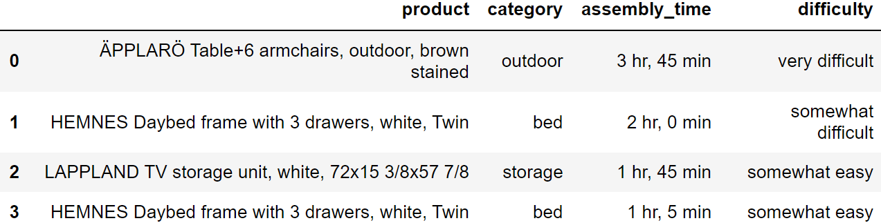
app_dataAn IKEA fan created an app where people can log the amount of time it
took them to assemble their IKEA furniture. The DataFrame
app_data has a row for each product build that was logged
on the app. The columns are:
'product' (str): the name of the product,
which includes the product line as the first word, followed by a
description of the product'category' (str): a categorical
description of the type of product'assembly_time' (str): the amount of time
to assemble the product, formatted as 'x hr, y min' where
x and y represent integers, possibly zero'minutes' (int): integer values
representing the number of minutes it took to assemble each productThe first few rows of app_data are shown below, though
app_data has many more rows than pictured (5000 rows
total).
Assume that we have already run import babypandas as bpd
and import numpy as np.
Tip: Open this page in another tab, so that it is easy to refer to this data description as you work through the exam.
Complete the expression below so that it evaluates to the name of the product for which the average assembly cost per package is lowest.
(ikea.assign(assembly_per_package = ___(a)___)
.sort_values(by='assembly_per_package').___(b)___)What goes in blank (a)?
Answer:
ikea.get('assembly_cost')/ikea.get('packages')
This column, as its name suggests, contains the average assembly cost per package, obtained by dividing the total cost of each product by the number of packages that product comes in. This code uses the fact that arithmetic operations between two Series happens element-wise.
The average score on this problem was 91%.
What goes in blank (b)?
Answer: get('product').iloc[0]
After adding the 'assembly_per_package' column and
sorting by that column in the default ascending order, the product with
the lowest 'assembly_per_package' will be in the very first
row. To access the name of that product, we need to get the
column containing product names and use iloc to access an
element of that Series by integer position.
The average score on this problem was 66%.
Complete the expression below so that it evaluates to a DataFrame
indexed by 'category' with one column called
'price' containing the median cost of the products in each
category.
ikea.___(a)___.get(___(b)___)What goes in blank (a)?
Answer:
groupby('category').median()
The question prompt says that the resulting DataFrame should be
indexed by 'category', so this is a hint that we may want
to group by 'category'. When using groupby, we
need to specify an aggregation function, and since we’re looking for the
median cost of all products in a category, we use the
.median() aggregation function.
The average score on this problem was 90%.
What goes in blank (b)?
Answer: ['price']
The question prompt also says that the resulting DataFrame should
have just one column, the 'price' column. To keep only
certain columns in a DataFrame, we use .get, passing in a
list of columns to keep. Remember to include the square brackets,
otherwise .get will return a Series instead of a
DataFrame.
The average score on this problem was 76%.
In the ikea DataFrame, the first word of each string in
the 'product' column represents the product line. For
example the HEMNES line of products includes several different products,
such as beds, dressers, and bedside tables.
The code below assigns a new column to the ikea
DataFrame containing the product line associated with each product.
(ikea.assign(product_line = ikea.get('product')
.apply(extract_product_line)))What are the input and output types of the
extract_product_line function?
takes a string as input, returns a string
takes a string as input, returns a Series
takes a Series as input, returns a string
takes a Series as input, returns a Series
Answer: takes a string as input, returns a string
To use the Series method .apply, we first need a Series,
containing values of any type. We pass in the name of a function to
.apply and essentially, .apply calls the given
function on each value of the Series, producing a Series with the
resulting outputs of those function calls. In this case,
.apply(extract_product_line) is called on the Series
ikea.get('product'), which contains string values. This
means the function extract_product_line must take strings
as inputs. We’re told that the code assigns a new column to the
ikea DataFrame containing the product line associated with
each product, and we know that the product line is a string, as it’s the
first word of the product name. This means the function
extract_product_line must output a string.
The average score on this problem was 72%.
Complete the return statement in the
extract_product_line function below.
def extract_product_line(x):
    return _________
What goes in the blank?
Answer: x.split(' ')[0]
This function should take as input a string x,
representing a product name, and return the first word of that string,
representing the product line. Since words are separated by spaces, we
want to split the string on the space character ' '.
It’s also correct to answer x.split()[0] without
specifying to split on spaces, because the default behavior of the
string .split method is to split on any whitespace, which
includes any number of spaces, tabs, newlines, etc. Since we’re only
extracting the first word, which will be separated from the rest of the
product name by a single space, it’s equivalent to split using single
spaces and using the default of any whitespace.
The average score on this problem was 84%.
Recall that we have the complete set of currently available discounts
in the DataFrame offers.
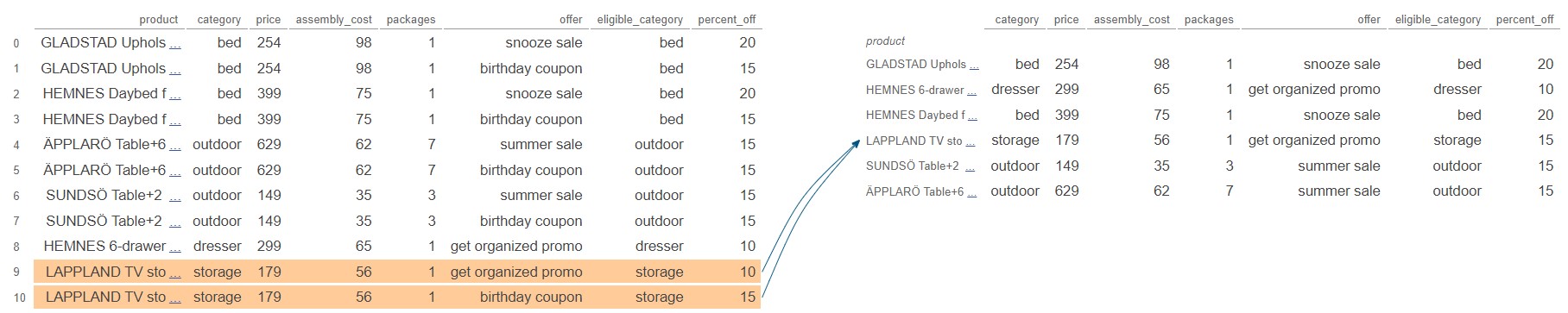
The DataFrame with_offers is created as follows.
    (with_offers = ikea.take(np.arange(6))
                       .merge(offers, left_on='category',
right_on='eligible_category'))How many rows does with_offers have?
Answer: 11
First, consider the DataFrame ikea.take(np.arange(6)),
which contains the first six rows of ikea. We know the
contents of these first six rows from the preview of the DataFrame at
the start of this exam. To merge with offers, we need to
look at the 'category' of each of these six rows and see
how many rows of offers have the same value in the
'eligible_category' column.
The first row of ikea.take(np.arange(6)) is a
'bed'. There are two 'bed' offers, so that
will create two rows in the output DataFrame. Similarly, the second row
of ikea.take(np.arange(6)) creates two rows in the output
DataFrame because there are two 'outdoor' offers. The third
row creates just one row in the output, since there is only one
'dresser' offer. Continuing row-by-row in this way, we can
sum the number of rows created to get: 2+2+1+2+2+2 = 11.
Pandas Tutor is a really helpful tool to visualize the merge process. Below is a color-coded visualization of this merge, generated by the code here.
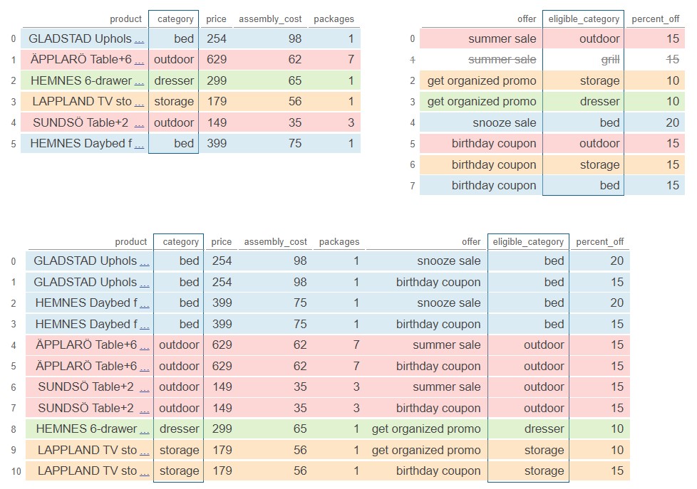
The average score on this problem was 41%.
How many rows of with_offers have a value of 20 in the
'percent_off' column?
Answer: 2
There is just one offer with a value of 20 in the
'percent_off' column, and this corresponds to an offer on a
'bed'. Since there are two rows of
ikea.take(np.arange(6)) with a 'category' of
'bed', each of these will match with the 20 percent-off
offer, creating two rows of with_offers with a value of 20
in the 'percent_off' column.
The
visualization
from Pandas Tutor below confirms our answer. The two rows with a
value of 20 in the 'percent_off' column are both shown in
rows 0 and 2 of the output DataFrame.
The average score on this problem was 70%.
If you can use just one offer per product, you’d want to use the one that saves you the most money, which we’ll call the best offer.
True or False: The expression below evaluates to a
Series indexed by 'product' with the name of the best offer
for each product that appears in the with_offers
DataFrame.
with_offers.groupby('product').max().get('offer')True
False
Answer: False
Recall that groupby applies the aggregation function
separately to each column. Applying the .max() aggregate on
the 'offer' column for each group gives the name that is
latest in alphabetical order because it contains strings, whereas
applying the .max() aggregate on the
'percent_off' column gives the largest numerical value.
These don’t necessarily go together in with_offers.
In particular, the element of
with_offers.groupby('product').max().get('offer')
corresponding to the LAPPLAND TV storage unit will be
'get_organized_promo'. This happens because the two rows of
with_offers corresponding to the LAPPLAND TV storage unit
have values of 'get_organized_promo' and
'birthday coupon', but 'get_organized_promo'
is alphabetically later, so it’s considered the max by
.groupby. However, the 'birthday coupon' is
actually a better offer, since it’s 15 percent off, while the
'get_organized_promo' is only 10 percent off. The
expression does not actually find the best offer for each product, but
instead finds the latest alphabetical offer for each product.
We can see this directly by looking at the output of Pandas Tutor below, generated by this code.
The average score on this problem was 69%.
You want to add a column to with_offers containing the
price after the offer discount is applied.
with_offers = with_offers.assign(after_price = _________)
with_offers
Which of the following could go in the blank? Select all that apply.
with_offers.get('price') - with_offers.get('percent_off')/100
with_offers.get('price')*(100 - with_offers.get('percent_off'))/100
with_offers.get('price') - with_offers.get('price')*with_offers.get('percent_off')/100
with_offers.get('price')*(100 - with_offers.get('percent_off')/100)
Answer:
with_offers.get('price')*(100 - with_offers.get('percent_off'))/100,
(with_offers.get('price') - with_offers.get('price')*with_offers.get('percent_off')/100)
Notice that all the answer choices use
with_offers.get('price'), which is a Series of prices, and
with_offers.get('percent_off'), which is a Series of
associated percentages off. Using Series arithmetic, which works
element-wise, the goal is to create a Series of prices after the
discount is applied.
For example, the first row of with_offers corresponds to
an item with a price of 254 dollars, and a discount of 20 percent off,
coming from the snooze sale. This means its price after the discount
should be 80 percent of the original value, which is 254*0.8 = 203.2 dollars.
Let’s go through each answer in order, working with this example.
The first answer choice takes the price and subtracts the percent off divided by 100. For our example, this would compute the discounted price as 254 - 20/100 = 253.8 dollars, which is incorrect.
The second answer choice multiplies the price by the quantity 100 minus the percent off, then divides by 100. This works because when we subtract the percent off from 100 and divide by 100, the result represents the proportion or fraction of the cost we must pay, and so multiplying by the price gives the price after the discount. For our example, this comes out to 254*(100-20)/100= 203.2 dollars, which is correct.
The third answer choice is also correct. This corresponds to taking the original price and subtracting from it the dollar amount off, which comes from multiplying the price by the percent off and dividing by 100. For our example, this would be computed as 254 - 254*20/100 = 203.2 dollars, which is correct.
The fourth answer multiplies the price by the quantity 100 minus the percent off divided by 100. For our example, this would compute the discounted price as 254*(100 - 20/100) = 25349.2 dollars, a number that’s nearly one hundred times the original price!
Therefore, only the second and third answer choices are correct.
The average score on this problem was 79%.
Recall that an IKEA fan created an app for people to log the amount
of time it takes them to assemble an IKEA product. We have this data in
app_data.
Suppose that when someone downloads the app, the app requires them to choose a username, which must be different from all other registered usernames.
True or False: If app_data had included
a column with the username of the person who reported each product
build, it would make sense to index app_data by
username.
True
False
Answer: False
Even though people must have distinct usernames, one person can build
multiple different IKEA products and log their time for each build. So
we don’t expect every row of app_data to have a distinct
username associated with it, and therefore username would not be
suitable as an index, since the index should have distinct values.
The average score on this problem was 52%.
What does the code below evaluate to?
(app_data.take(np.arange(4))
         .sort_values(by='assembly_time')
         .get('assembly_time')
         .iloc[0])
Hint: The 'assembly_time' column contains
strings.
Answer: '1 hr, 45 min'
The code says that we should take the first four rows of
app_data (which we can see in the preview at the start of
this exam), sort the rows in ascending order of
'assembly_time', and extract the very first entry of the
'assembly_time' column. In other words, we have to find the
'assembly_time' value that would be first when sorted in
ascending order. As given in the hint, the 'assembly_time'
column contains strings, and strings get sorted alphabetically, so we
are looking for the assembly time, among the first four, that would come
first alphabetically. This is '1 hr, 45 min'.
Note that first alphabetically does not correspond to the least
amount of time. '1 hr, 5 min' represents less time than
'1 hr, 45 min', but in alphabetical order
'1 hr, 45 min' comes before '1 hr, 5 min'
because both start with the same characters '1 hr, ' and
comparing the next character, '4' comes before
'5'.
The average score on this problem was 46%.
Complete the implementation of the to_minutes function
below. This function takes as input a string formatted as
'x hr, y min' where x and y
represent integers, and returns the corresponding number of minutes,
as an integer (type int in Python).
For example, to_minutes('3 hr, 5 min') should return
185.
def to_minutes(time):
    first_split = time.split(' hr, ')
    second_split = first_split[1].split(' min')
    return _________
What goes in the blank?
Answer:
int(first_split[0])*60+int(second_split[0])
As the last subpart demonstrated, if we want to compare times, it
doesn’t make sense to do so when times are represented as strings. In
the to_minutes function, we convert a time string into an
integer number of minutes.
The first step is to understand the logic. Every hour contains 60
minutes, so for a time string formatted like x hr, y min'
the total number of minutes comes from multiplying the value of
x by 60 and adding y.
The second step is to understand how to extract the x
and y values from the time string using the string methods
.split. The string method .split takes as
input some separator string and breaks the string into pieces at each
instance of the separator string. It then returns a list of all those
pieces. The first line of code, therefore, creates a list called
first_split containing two elements. The first element,
accessed by first_split[0] contains the part of the time
string that comes before ' hr, '. That is,
first_split[0] evaluates to the string x.
Similarly, first_split[1] contains the part of the time
string that comes after ' hr, '. So it is formatted like
'y min'. If we split this string again using the separator
of ' min', the result will be a list whose first element is
the string 'y'. This list is saved as
second_split so second_split[0] evaluates to
the string y.
Now we have the pieces we need to compute the number of minutes,
using the idea of multiplying the value of x by 60 and
adding y. We have to be careful with data types here, as
the bolded instructions warn us that the function must return an
integer. Right now, first_split[0] evaluates to the string
x and second_split[0] evaluates to the string
y. We need to convert these strings to integers before we
can multiply and add. Once we convert using the int
function, then we can multiply the number of hours by 60 and add the
number of minutes. Therefore, the solution is
int(first_split[0])*60+int(second_split[0]).
Note that failure to convert strings to integers using the
int function would lead to very different behavior. Let’s
take the example time string of '3 hr, 5 min' as input to
our function. With the return statement as
int(first_split[0])*60+int(second_split[0]), the function
would return 185 on this input, as desired. With the return statement as
first_split[0]*60+second_split[0], the function would
return a string of length 61, looking something like this
'3333...33335'. That’s because the * and
+ symbols do have meaning for strings, they’re just
different meanings than when used with integers.
The average score on this problem was 71%.
You want to add to app_data a column called
'minutes' with integer values representing the number of
minutes it took to assemble each product.
app_data = app_data.assign(minutes = _________)
app_data
Which of the following should go in the blank?
to_minutes('assembly_time')
to_minutes(app_data.get('assembly_time'))
app_data.get('assembly_time').apply(to_minutes)
app_data.get('assembly_time').apply(to_minutes(time))
Answer:
app_data.get('assembly_time').apply(to_minutes)
We want to create a Series of times in minutes, since it’s to be
added to the app_data DataFrame using .assign.
The correct way to do that is to use .apply so that our
function, which works for one input time string, can be applied
separately to every time string in the 'assembly_time'
column of app_data. Remember that .apply takes
as input one parameter, the name of the function to apply, with no
arguments. The correct syntax is
app_data.get('assembly_time').apply(to_minutes).
The average score on this problem was 98%.
We want to use app_data to estimate the average amount
of time it takes to build an IKEA bed (any product in the
'bed' category). Which of the following strategies would be
an appropriate way to estimate this quantity? Select all that apply.
Query to keep only the beds. Then resample with replacement many
times. For each resample, take the mean of the 'minutes'
column. Compute a 95% confidence interval based on those means.
Query to keep only the beds. Group by 'product' using
the mean aggregation function. Then resample with replacement many
times. For each resample, take the mean of the 'minutes'
column. Compute a 95% confidence interval based on those means.
Resample with replacement many times. For each resample, first query
to keep only the beds and then take the mean of the
'minutes' column. Compute a 95% confidence interval based
on those means.
Resample with replacement many times. For each resample, first query
to keep only the beds. Then group by 'product' using the
mean aggregation function, and finally take the mean of the
'minutes' column. Compute a 95% confidence interval based
on those means.
Answer: Option 1
Only the first answer is correct. This is a question of parameter estimation, so our approach is to use bootstrapping to create many resamples of our original sample, computing the average of each resample. Each resample should always be the same size as the original sample. The first answer choice accomplishes this by querying first to keep only the beds, then resampling from the DataFrame of beds only. This means resamples will have the same size as the original sample. Each resample’s mean will be computed, so we will have many resample means from which to construct our 95% confidence interval.
In the second answer choice, we are actually taking the mean twice.
We first average the build times for all builds of the same product when
grouping by product. This produces a DataFrame of different products
with the average build time for each. We then resample from this
DataFrame, computing the average of each resample. But this is a
resample of products, not of product builds. The size of the resample is
the number of unique products in app_data, not the number
of reported product builds in app_data. Further, we get
incorrect results by averaging numbers that are already averages. For
example, if 5 people build bed A and it takes them each 1 hour, and 1
person builds bed B and it takes them 10 hours, the average amount of
time to build a bed is \frac{5*1+10}{6} =
2.5. But if we average the times for bed A (1 hour) and average
the times for bed B (5 hours), then average those, we get \frac{1+5}{2} = 3, which is not the same.
More generally, grouping is not a part of the bootstrapping process
because we want each data value to be weighted equally.
The last two answer choices are incorrect because they involve
resampling from the full app_data DataFrame before querying
to keep only the beds. This is incorrect because it does not preserve
the sample size. For example, if app_data contains 1000
reported bed builds and 4000 other product builds, then the only
relevant data is the 1000 bed build times, so when we resample, we want
to consider another set of 1000 beds. If we resample from the full
app_data DataFrame, our resample will contain 5000 rows,
but the number of beds will be random, not necessarily 1000. If we query
first to keep only the beds, then resample, our resample will contain
exactly 1000 beds every time. As an added bonus, since we only care
about beds, it’s much faster to resample from a smaller DataFrame of
beds only than it is to resample from all app_data with
plenty of rows we don’t care about.
The average score on this problem was 71%.
Laura built the LAPPLAND TV storage unit in 2 hours and 30 minutes,
and she thinks she worked at an average speed. If you want to see
whether the average time to build the TV storage unit is indeed 2 hours
and 30 minutes using the sample of assembly times in
app_data, which of the following tools
could you use to help you? Select all that apply.
hypothesis testing
permutation testing
bootstrapping
Central Limit Theorem
confidence interval
regression
Answer: hypothesis testing, bootstrapping, Central Limit Theorem, confidence interval
The average time to build the LAPPLAND TV storage unit is an unknown population parameter. We’re trying to figure out if this parameter could be equal to the specific value of 2 hours and 30 minutes. We can use the framework we learned in class to set this up as a hypothesis test via confidence interval. When we have a null hypothesis of the form “the parameter equals the specific value” and an alternative hypothesis of “it does not,” this framework applies, and conducting the hypothesis test is equivalent to constructing a confidence interval for the parameter and seeing if the specific value falls in the interval.
There are two ways in which we could construct the confidence interval. One is through bootstrapping, and the other is through the Central Limit Theorem, which applies in this case because our statistic is the mean.
The only listed tools that could not be used here are permutation testing and regression. Permutation testing is used to determine whether two samples could have come from the same population, but here we only have one sample. Permutation testing would be helpful to answer a question like, “Does it take the same amount of time to assemble the LAPPLAND TV storage as it does to assemble the HAUGA TV storage unit?”
Regression is used to predict one numerical quantity based on another, not to estimate a parameter as we are doing here. Regression would be appropriate to answer a question like, “How does the assembly time for the LAPPLAND TV storage unit change with the assembler’s age?”
The average score on this problem was 78%.
For this question, let’s think of the data in app_data
as a random sample of all IKEA purchases and use it to test the
following hypotheses.
Null Hypothesis: IKEA sells an equal amount of beds
(category 'bed') and outdoor furniture (category
'outdoor').
Alternative Hypothesis: IKEA sells more beds than outdoor furniture.
The DataFrame app_data contains 5000 rows, which form
our sample. Of these 5000 products,
Which of the following could be used as the test statistic for this hypothesis test? Select all that apply.
Among 2500 beds and outdoor furniture items, the absolute difference between the proportion of beds and the proportion of outdoor furniture.
Among 2500 beds and outdoor furniture items, the proportion of beds.
Among 2500 beds and outdoor furniture items, the number of beds.
Among 2500 beds and outdoor furniture items, the number of beds plus the number of outdoor furniture items.
Answer: Among 2500 beds and outdoor furniture
items, the proportion of beds.
Among 2500 beds and outdoor
furniture items, the number of beds.
Our test statistic needs to be able to distinguish between the two hypotheses. The first option does not do this, because it includes an absolute value. If the absolute difference between the proportion of beds and the proportion of outdoor furniture were large, it could be because IKEA sells more beds than outdoor furniture, but it could also be because IKEA sells more outdoor furniture than beds.
The second option is a valid test statistic, because if the proportion of beds is large, that suggests that the alternative hypothesis may be true.
Similarly, the third option works because if the number of beds (out of 2500) is large, that suggests that the alternative hypothesis may be true.
The fourth option is invalid because out of 2500 beds and outdoor furniture items, the number of beds plus the number of outdoor furniture items is always 2500. So the value of this statistic is constant regardless of whether the alternative hypothesis is true, which means it does not help you distinguish between the two hypotheses.
The average score on this problem was 78%.
Let’s do a hypothesis test with the following test statistic: among 2500 beds and outdoor furniture items, the proportion of outdoor furniture minus the proportion of beds.
Complete the code below to calculate the observed value of the test
statistic and save the result as obs_diff.
    outdoor = (app_data.get('category')=='outdoor')
    bed = (app_data.get('category')=='bed')
    obs_diff = ( ___(a)___ - ___(b)___ ) / ___(c)___
The table below contains several Python expressions. Choose the correct expression to fill in each of the three blanks. Three expressions will be used, and two will be unused.
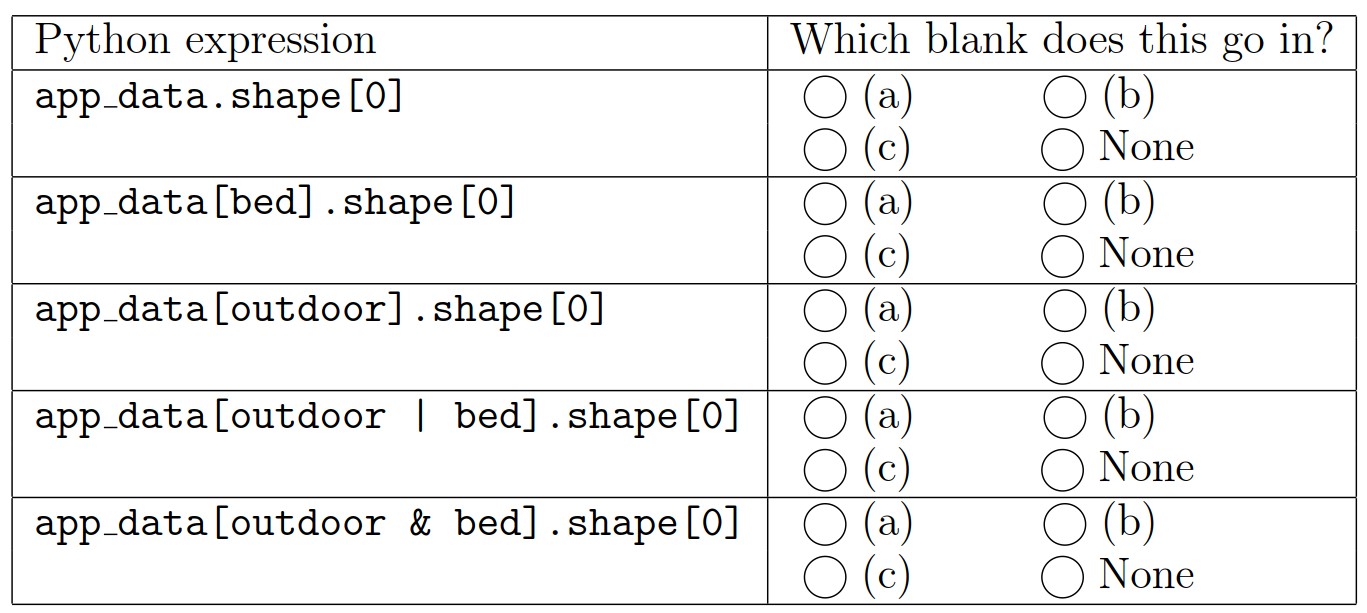
Answer: Reading the table from top to bottom, the five expressions should be used in the following blanks: None, (b), (a), (c), None.
The correct way to define obs_diff is
    outdoor = (app_data.get('category')=='outdoor')
    bed = (app_data.get('category')=='bed')
    obs_diff = (app_data[outdoor].shape[0] - app_data[bed].shape[0]) / app_data[outdoor | bed].shape[0]
The first provided line of code defines a boolean Series called
outdoor with a value of True corresponding to
each outdoor furniture item in app_data. Using this as the
condition in a query results in a DataFrame of outdoor furniture items,
and using .shape[0] on this DataFrame gives the number of
outdoor furniture items. So app_data[outdoor].shape[0]
represents the number of outdoor furniture items in
app_data. Similarly, app_data[bed].shape[0]
represents the number of beds in app_data. Likewise,
app_data[outdoor | bed].shape[0] represents the total
number of outdoor furniture items and beds in app_data.
Notice that we need to use an or condition (|) to
get a DataFrame that contains both outdoor furniture and beds.
We are told that the test statistic should be the proportion of outdoor furniture minus the proportion of beds. Translating this directly into code, this means the test statistic should be calculated as
obs_diff = app_data[outdoor].shape[0]/app_data[outdoor | bed].shape[0] - app_data[bed].shape[0]) / app_data[outdoor | bed].shape[0]Since this is a difference of two fractions with the same denominator, we can equivalently subtract the numerators first, then divide by the common denominator, using the mathematical fact \frac{a}{c} - \frac{b}{c} = \frac{a-b}{c}.
This yields the answer
obs_diff = (app_data[outdoor].shape[0] - app_data[bed].shape[0]) / app_data[outdoor | bed].shape[0]Notice that this is the observed value of the test statistic
because it’s based on the real-life data in the app_data
DataFrame, not simulated data.
The average score on this problem was 90%.
Which of the following is a valid way to generate one value of the test statistic according to the null model? Select all that apply.
Way 1:
multi = np.random.multinomial(2500, [0.5,0.5])
(multi[0] - multi[1])/2500
Way 2:
outdoor = np.random.multinomial(2500, [0.5,0.5])[0]/2500
bed = np.random.multinomial(2500, [0.5,0.5])[1]/2500
outdoor - bed
Way 3:
choice = np.random.choice([0, 1], 2500, replace=True)
choice_sum = choice.sum()
(choice_sum - (2500 - choice_sum))/2500
Way 4:
choice = np.random.choice(['bed', 'outdoor'], 2500, replace=True)
bed = np.count_nonzero(choice=='bed')
outdoor = np.count_nonzero(choice=='outdoor')
outdoor/2500 - bed/2500
Way 5:
outdoor = (app_data.get('category')=='outdoor')
bed = (app_data.get('category')=='bed')
samp = app_data[outdoor|bed].sample(2500, replace=True)
samp[samp.get('category')=='outdoor'].shape[0]/2500 -  samp[samp.get('category')=='bed'].shape[0]/2500)
Way 6:
outdoor = (app_data.get('category')=='outdoor')
bed = (app_data.get('category')=='bed')
samp = (app_data[outdoor|bed].groupby('category').count().reset_index().sample(2500, replace=True))
samp[samp.get('category')=='outdoor'].shape[0]/2500 - samp[samp.get('category')=='bed'].shape[0]/2500
Way 1
Way 2
Way 3
Way 4
Way 5
Way 6
Answer: Way 1, Way 3, Way 4, Way 6
Let’s consider each way in order.
Way 1 is a correct solution. This code begins by defining a variable
multi which will evaluate to an array with two elements
representing the number of items in each of the two categories, after
2500 items are drawn randomly from the two categories, with each
category being equally likely. In this case, our categories are beds and
outdoor furniture, and the null hypothesis says that each category is
equally likely, so this describes our scenario accurately. We can
interpret multi[0] as the number of outdoor furniture items
and multi[1] as the number of beds when we draw 2500 of
these items with equal probability. Using the same mathematical fact
from the solution to Problem 8.2, we can calculate the difference in
proportions as the difference in number divided by the total, so it is
correct to calculate the test statistic as
(multi[0] - multi[1])/2500.
Way 2 is an incorrect solution. Way 2 is based on a similar idea as
Way 1, except it calls np.random.multinomial twice, which
corresponds to two separate random processes of selecting 2500 items,
each of which is equally likely to be a bed or an outdoor furniture
item. However, is not guaranteed that the number of outdoor furniture
items in the first random selection plus the number of beds in the
second random selection totals 2500. Way 2 calculates the proportion of
outdoor furniture items in one random selection minus the proportion of
beds in another. What we want to do instead is calculate the difference
between the proportion of outdoor furniture and beds in a single random
draw.
Way 3 is a correct solution. Way 3 does the random selection of items
in a different way, using np.random.choice. Way 3 creates a
variable called choice which is an array of 2500 values.
Each value is chosen from the list [0,1] with each of the
two list elements being equally likely to be chosen. Of course, since we
are choosing 2500 items from a list of size 2, we must allow
replacements. We can interpret the elements of choice by
thinking of each 1 as an outdoor furniture item and each 0 as a bed. By
doing so, this random selection process matches up with the assumptions
of the null hypothesis. Then the sum of the elements of
choice represents the total number of outdoor furniture
items, which the code saves as the variable choice_sum.
Since there are 2500 beds and outdoor furniture items in total,
2500 - choice_sum represents the total number of beds.
Therefore, the test statistic here is correctly calculated as the number
of outdoor furniture items minus the number of beds, all divided by the
total number of items, which is 2500.
Way 4 is a correct solution. Way 4 is similar to Way 3, except
instead of using 0s and 1s, it uses the strings 'bed' and
'outdoor' in the choice array, so the
interpretation is even more direct. Another difference is the way the
number of beds and number of outdoor furniture items is calculated. It
uses np.count_nonzero instead of sum, which wouldn’t make
sense with strings. This solution calculates the proportion of outdoor
furniture minus the proportion of beds directly.
Way 5 is an incorrect solution. As described in the solution to
Problem 8.2, app_data[outdoor|bed] is a DataFrame
containing just the outdoor furniture items and the beds from
app_data. Based on the given information, we know
app_data[outdoor|bed] has 2500 rows, 1000 of which
correspond to beds and 1500 of which correspond to furniture items. This
code defines a variable samp that comes from sampling this
DataFrame 2500 times with replacement. This means that each row of
samp is equally likely to be any of the 2500 rows of
app_data[outdoor|bed]. The fraction of these rows that are
beds is 1000/2500 = 2/5 and the
fraction of these rows that are outdoor furniture items is 1500/2500 = 3/5. This means the random
process of selecting rows randomly such that each row is equally likely
does not make each item equally likely to be a bed or outdoor furniture
item. Therefore, this approach does not align with the assumptions of
the null hypothesis.
Way 6 is a correct solution. Way 6 essentially modifies Way 5 to make
beds and outdoor furniture items equally likely to be selected in the
random sample. As in Way 5, the code involves the DataFrame
app_data[outdoor|bed] which contains 1000 beds and 1500
outdoor furniture items. Then this DataFrame is grouped by
'category' which results in a DataFrame indexed by
'category', which will have only two rows, since there are
only two values of 'category', either
'outdoor' or 'bed'. The aggregation function
.count() is irrelevant here. When the index is reset,
'category' becomes a column. Now, randomly sampling from
this two-row grouped DataFrame such that each row is equally likely to
be selected does correspond to choosing items such that each
item is equally likely to be a bed or outdoor furniture item. The last
line simply calculates the proportion of outdoor furniture items minus
the proportion of beds in our random sample drawn according to the null
model.
The average score on this problem was 59%.
Suppose we generate 10,000 simulated values of the test statistic
according to the null model and store them in an array called
simulated_diffs. Complete the code below to calculate the
p-value for the hypothesis test.
np.count_nonzero(simulated_diffs _________ obs_diff)/10000What goes in the blank?
<
<=
>
>=
Answer: <=
To answer this question, we need to know whether small values or large values of the test statistic indicate the alternative hypothesis. The alternative hypothesis is that IKEA sells more beds than outdoor furniture. Since we’re calculating the proportion of outdoor furniture minus the proportion of beds, this difference will be small (negative) if the alternative hypothesis is true. Larger (positive) values of the test statistic mean that IKEA sells more outdoor furniture than beds. A value near 0 means they sell beds and outdoor furniture equally.
The p-value is defined as the proportion of simulated test statistics
that are equal to the observed value or more extreme, where extreme
means in the direction of the alternative. In this case, since small
values of the test statistic indicate the alternative hypothesis, the
correct answer is <=.
The average score on this problem was 43%.
You are browsing the IKEA showroom, deciding whether to purchase the
BILLY bookcase or the LOMMARP bookcase. You are concerned about the
amount of time it will take to assemble your new bookcase, so you look
up the assembly times reported in app_data. Thinking of the
data in app_data as a random sample of all IKEA purchases,
you want to perform a permutation test to test the following
hypotheses.
Null Hypothesis: The assembly time for the BILLY bookcase and the assembly time for the LOMMARP bookcase come from the same distribution.
Alternative Hypothesis: The assembly time for the BILLY bookcase and the assembly time for the LOMMARP bookcase come from different distributions.
Suppose we query app_data to keep only the BILLY
bookcases, then average the 'minutes' column. In addition,
we separately query app_data to keep only the LOMMARP
bookcases, then average the 'minutes' column. If the null
hypothesis is true, which of the following statements about these two
averages is correct?
These two averages are the same.
Any difference between these two averages is due to random chance.
Any difference between these two averages cannot be ascribed to random chance alone.
The difference between these averages is statistically significant.
Answer: Any difference between these two averages is due to random chance.
If the null hypothesis is true, this means that the time recorded in
app_data for each BILLY bookcase is a random number that
comes from some distribution, and the time recorded in
app_data for each LOMMARP bookcase is a random number that
comes from the same distribution. Each assembly time is a
random number, so even if the null hypothesis is true, if we take one
person who assembles a BILLY bookcase and one person who assembles a
LOMMARP bookcase, there is no guarantee that their assembly times will
match. Their assembly times might match, or they might be different,
because assembly time is random. Randomness is the only reason that
their assembly times might be different, as the null hypothesis says
there is no systematic difference in assembly times between the two
bookcases. Specifically, it’s not the case that one typically takes
longer to assemble than the other.
With those points in mind, let’s go through the answer choices.
The first answer choice is incorrect. Just because two sets of
numbers are drawn from the same distribution, the numbers themselves
might be different due to randomness, and the averages might also be
different. Maybe just by chance, the people who assembled the BILLY
bookcases and recorded their times in app_data were slower
on average than the people who assembled LOMMARP bookcases. If the null
hypothesis is true, this difference in average assembly time should be
small, but it very likely exists to some degree.
The second answer choice is correct. If the null hypothesis is true, the only reason for the difference is random chance alone.
The third answer choice is incorrect for the same reason that the second answer choice is correct. If the null hypothesis is true, any difference must be explained by random chance.
The fourth answer choice is incorrect. If there is a difference between the averages, it should be very small and not statistically significant. In other words, if we did a hypothesis test and the null hypothesis was true, we should fail to reject the null.
The average score on this problem was 77%.
For the permutation test, we’ll use as our test statistic the average assembly time for BILLY bookcases minus the average assembly time for LOMMARP bookcases, in minutes.
Complete the code below to generate one simulated value of the test
statistic in a new way, without using
np.random.permutation.
billy = (app_data.get('product') ==
        'BILLY Bookcase, white, 31 1/2x11x79 1/2')
lommarp = (app_data.get('product') ==
          'LOMMARP Bookcase, dark blue-green, 25 5/8x78 3/8')
billy_lommarp = app_data[billy|lommarp]
billy_mean = np.random.choice(billy_lommarp.get('minutes'), billy.sum(), replace=False).mean()
lommarp_mean = _________
billy_mean - lommarp_mean
What goes in the blank?
billy_lommarp[lommarp].get('minutes').mean()
np.random.choice(billy_lommarp.get('minutes'), lommarp.sum(), replace=False).mean()
billy_lommarp.get('minutes').mean() - billy_mean
(billy_lommarp.get('minutes').sum() - billy_mean * billy.sum())/lommarp.sum()
Answer:
(billy_lommarp.get('minutes').sum() - billy_mean * billy.sum())/lommarp.sum()
The first line of code creates a boolean Series with a True value for
every BILLY bookcase, and the second line of code creates the analogous
Series for the LOMMARP bookcase. The third line queries to define a
DataFrame called billy_lommarp containing all products that
are BILLY or LOMMARP bookcases. In other words, this DataFrame contains
a mix of BILLY and LOMMARP bookcases.
From this point, the way we would normally proceed in a permutation
test would be to use np.random.permutation to shuffle one
of the two relevant columns (either 'product' or
'minutes') to create a random pairing of assembly times
with products. Then we would calculate the average of all assembly times
that were randomly assigned to the label BILLY. Similarly, we’d
calculate the average of all assembly times that were randomly assigned
to the label LOMMARP. Then we’d subtract these averages to get one
simulated value of the test statistic. To run the permutation test, we’d
have to repeat this process many times.
In this problem, we need to generate a simulated value of the test
statistic, without randomly shuffling one of the columns. The code
starts us off by defining a variable called billy_mean that
comes from using np.random.choice. There’s a lot going on
here, so let’s break it down. Remember that the first argument to
np.random.choice is a sequence of values to choose from,
and the second is the number of random choices to make. And we set
replace=False, so that no element that has already been
chosen can be chosen again. Here, we’re making our random choices from
the 'minutes' column of billy_lommarp. The
number of choices to make from this collection of values is
billy.sum(), which is the sum of all values in the
billy Series defined in the first line of code. The
billy Series contains True/False values, but in Python,
True counts as 1 and False counts as 0, so billy.sum()
evaluates to the number of True entries in billy, which is
the number of BILLY bookcases recorded in app_data. It
helps to think of the random process like this:
If we think of the random times we draw as being labeled BILLY, then the remaining assembly times still leftover in the bag represent the assembly times randomly labeled LOMMARP. In other words, this is a random association of assembly times to labels (BILLY or LOMMARP), which is the same thing we usually accomplish by shuffling in a permutation test.
From here, we can proceed the same way as usual. First, we need to
calculate the average of all assembly times that were randomly assigned
to the label BILLY. This is done for us and stored in
billy_mean. We also need to calculate the average of all
assembly times that were randomly assigned the label LOMMARP. We’ll call
that lommarp_mean. Thinking of picking times out of a large
bag, this is the average of all the assembly times left in the bag. The
problem is there is no easy way to access the assembly times that were
not picked. We can take advantage of the fact that we can easily
calculate the total assembly time of all BILLY and LOMMARP bookcases
together with billy_lommarp.get('minutes').sum(). Then if
we subtract the total assembly time of all bookcases randomly labeled
BILLY, we’ll be left with the total assembly time of all bookcases
randomly labeled LOMMARP. That is,
billy_lommarp.get('minutes').sum() - billy_mean * billy.sum()
represents the total assembly time of all bookcases randomly labeled
LOMMARP. The count of the number of LOMMARP bookcases is given by
lommarp.sum() so the average is
(billy_lommarp.get('minutes').sum() - billy_mean * billy.sum())/lommarp.sum().
A common wrong answer for this question was the second answer choice,
np.random.choice(billy_lommarp.get('minutes'), lommarp.sum(), replace=False).mean().
This mimics the structure of how billy_mean was defined so
it’s a natural guess. However, this corresponds to the following random
process, which doesn’t associate each assembly with a unique label
(BILLY or LOMMARP):
We could easily get the same assembly time once for BILLY and once for LOMMARP, while other assembly times could get picked for neither. This process doesn’t split the data into two random groups as desired.
The average score on this problem was 12%.
IKEA is piloting a new rewards program where customers can earn free Swedish meatball plates from the in-store cafe when they purchase expensive items. Meatball plates are awarded as follows. Assume the item price is always an integer.
| Item price | Number of meatball plates |
|---|---|
| less than 99 dollars | 0 |
| 100 to 199 dollars | 1 |
| 200 dollars or more | 2 |
We want to implement a function called
calculate_meatball_plates that takes as input an array of
several item prices, corresponding to the individual items purchased in
one transaction, and returns the total number of meatball plates earned
in that transaction.
Select all correct ways of implementing this function from the options below.
Way 1:
def calculate_meatball_plates(prices):
    meatball_plates = 0
    for price in prices:
        if price >= 100 and price <= 199:
            meatball_plates = 1
        elif price >= 200:
            meatball_plates = 2
    return meatball_plates
Way 2:
def calculate_meatball_plates(prices):
    meatball_plates = 0
    for price in prices:
        if price >= 200:
            meatball_plates = meatball_plates + 1
        if price >= 100:
            meatball_plates = meatball_plates + 1
    return meatball_plates
Way 3:
def calculate_meatball_plates(prices):
    return np.count_nonzero(prices >= 100) + np.count_nonzero(prices >= 200)
Way 4:
def calculate_meatball_plates(prices):
    return (prices >= 200).sum()*2 + ((100 <= prices) & (prices <= 199)).sum()*1
Way 1
Way 2
Way 3
Way 4
Answer: Way 2, Way 3, Way 4
Way 1 does not work because it resets the variable
meatball_plates with each iteration instead of adding to a
running total. At the end of the loop, meatball_plates
evaluates to the number of meatball plates earned by the last price in
prices instead of the total number of meatball plates
earned by all purchases. A quick way to see this is incorrect is to
notice that the only possible return values are 0, 1, and 2, but it’s
possible to earn more than 2 meatball plates with enough purchases.
Way 2 works. As in Way 1, it loops through each price in
prices. When evaluating each price, it checks if the price
is at least 200 dollars, and if so, increments the total number of
meatball plates by 1. Then it checks if the price is at least 100
dollars, and if so, increments the count of meatball plates again. This
works because for prices that are at least 200 dollars, both
if conditions are satisfied, so the meatball plate count
goes up by 2, and for prices that are between 100 and 199 dollars, only
one of the if conditions is satisfied, so the count
increases by 1. For prices less than 100 dollars, the count doesn’t
change.
Way 3 works without using any iteration at all. It uses
np.count_nonzero to count the number of prices that are at
least 100 dollars, then it similarly counts the number of prices that
are at least 200 dollars and adds these together. This works because
prices that are at least 200 dollars are also at least 100 dollars, so
they contribute 2 to the total. Prices that are between 100 and 199
contribute 1, and prices below 100 dollars don’t contribute at all.
Way 4 also works and calculates the number of meatball plates without
iteration. The expression prices >= 200 evaluates to a
boolean Series with True for each price that is at least 200 dollars.
Summing this Series gives a count of the number of prices that are at
least 200 dollars, since True counts as 1 and False counts as 0 in
Python. Each such purchase earns 2 meatball plates, so this count of
purchases 200 dollars and up gets multiplied by 2. Similarly,
(100 <= prices) & (prices <= 199) is a Series
containing True for each price that is at least 100 dollars and at most
199 dollars, and the sum of that Series is the number of prices between
100 and 199 dollars. Each such purchase contributes one additional
meatball plate, so the number of such purchases gets multiplied by 1 and
added to the total.
The average score on this problem was 64%.
The histogram below shows the distribution of the number of products sold per day throughout the last 30 days, for two different IKEA products: the KURA reversible bed, and the ANTILOP highchair.
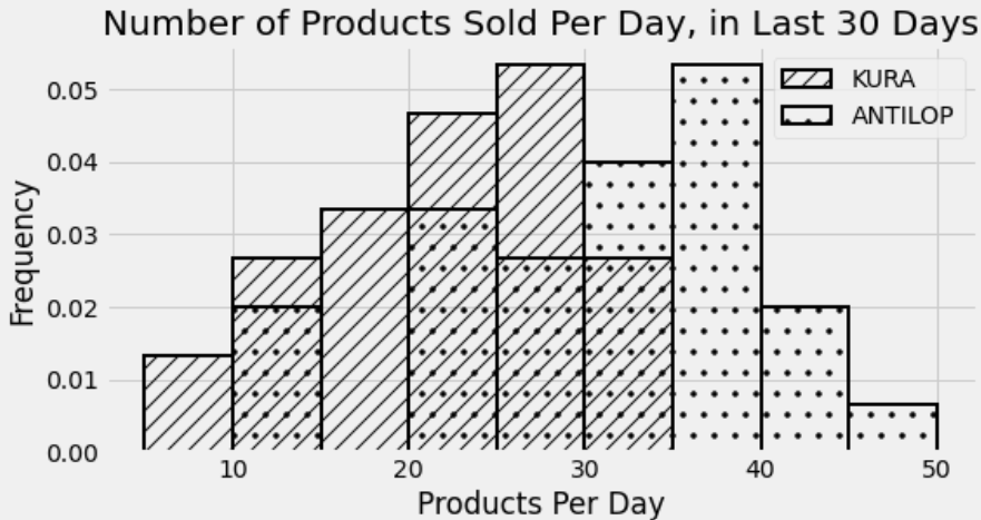
For how many days did IKEA sell between 20 (inclusive) and 30 (exclusive) KURA reversible beds per? Give an integer answer or write “not enough information”, but not both.
Answer: 15
Remember that for a density histogram, the proportion of data that falls in a certain range is the area of the histogram between those bounds. So to find the proportion of days for which IKEA sold between 20 and 30 KURA reversible beds, we need to find the total area of the bins [20, 25) and [25, 30). Note that the left endpoint of each bin is included and the right bin is not, which works perfectly with needing to include 20 and exclude 30.
The bin [20, 25) has a width of 5 and a height of about 0.047. The bin [25, 30) has a width of 5 and a height of about 0.053. The heights are approximate by eye, but it appears that the [20, 25) bin is below the horizontal line at 0.05 by the same amount which the [25, 30) is above that line. Noticing this spares us some annoying arithmetic and we can calculate the total area as
\begin{aligned} \text{total area} &= 5*0.047 + 5*0.053 \\ &= 5*(0.047 + 0.053) \\ &= 5*(0.1) \\ &= 0.5 \end{aligned}
Therefore, the proportion of days where IKEA sold between 20 and 30 KURA reversible beds is 0.5. Since there are 30 days represented in this histogram, that corresponds to 15 days.
The average score on this problem was 54%.
For how many days did IKEA sell more KURA reversible beds than ANTILOP highchairs? Give an integer answer or write “not enough information”, but not both.
Answer: not enough information
We cannot compare the number of KURA reversible beds sold on a certain day with the number of ANTILOP highchairs sold on the same day. These are two separate histograms shown on the same axes, but we have no way to associate data from one histogram with data from the other. For example, it’s possible that on some days, IKEA sold the same number of KURA reversible beds and ANTILOP highchairs. It’s also possible from this histogram that this never happened on any day.
The average score on this problem was 54%.
Determine the relative order of the three quantities below.
(1)<(2)<(3)
(1)<(3)<(2)
(2)<(1)<(3)
(2)<(3)<(1)
(3)<(1)<(2)
(3)<(2)<(1)
Answer: (2)<(3)<(1)
We can calculate the exact value of each of the quantities:
To find the number of days for which IKEA sold at least 35 ANTILOP highchairs, we need to find the total area of the rightmost three bins of the ANTILOP distribution. Doing a similar calculation to the one we did in Problem 11.1, \begin{aligned} \text{total area} &= 5*0.053 + 5*0.02 + 5*0.007 \\ &= 5*(0.08) \\ &= 0.4 \end{aligned} This is a proportion of 0.4 out of 30 days total, which corresponds to 12 days.
To find the number of days for which IKEA sold less than 25 ANTILOP highchairs, we need to find the total area of the leftmost four bins of the ANTILOP distribution. We can do this in the same way as before, but to avoid the math, we can also use the information we’ve already figured out to make this easier. In Problem 11.1, we learned that the KURA distribution included 15 days total in the two bins [20, 25) and [25, 30). Since the [25, 30) bin is just slightly taller than the [20, 25) bin, these 15 days must be split as 7 in the [20, 25) bin and 8 in the [25, 30) bin. Once we know the tallest bin corresponds to 8 days, we can figure out the number of days corresponding to every other bin just by eye. Anything that’s half as tall as the tallest bin, for example, represents 4 days. The red lines on the histogram below each represent 1 day, so we can easily count the number of days in each bin.
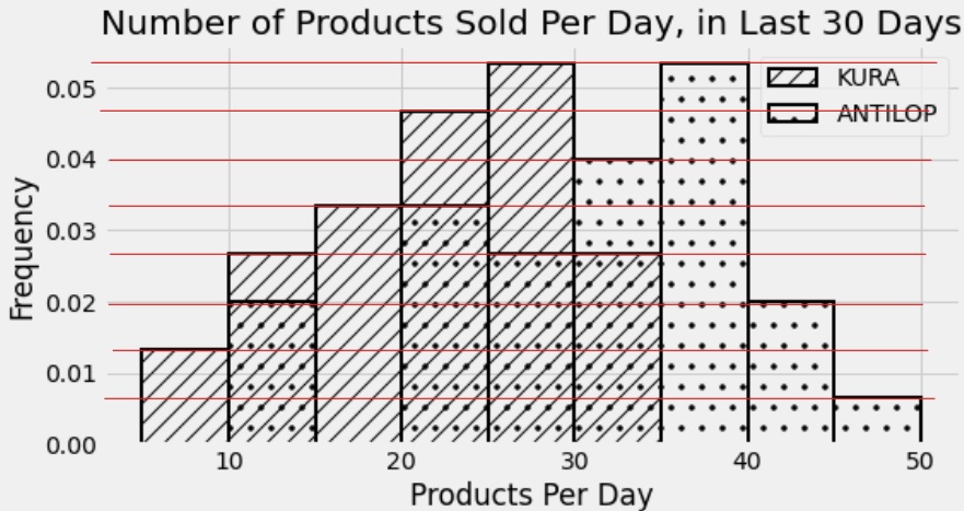
To find the number of days for which IKEA sold between 10 and 20 KURA reversible beds, we simply need to add the number of days in the [10, 15) and [15, 20) bins of the KURA distribution. Using the histogram with the red lines makes this easy to calculate as 4+5, or 9 days.
Therefore since 8<9<12, the correct answer is (2)<(3)<(1).
The average score on this problem was 81%.
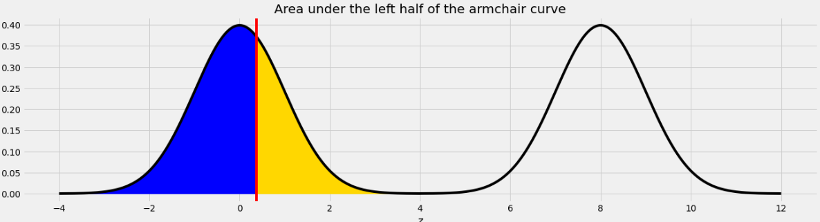
An IKEA chair designer is experimenting with some new ideas for armchair designs. She has the idea of making the arm rests shaped like bell curves, or normal distributions. A cross-section of the armchair design is shown below.
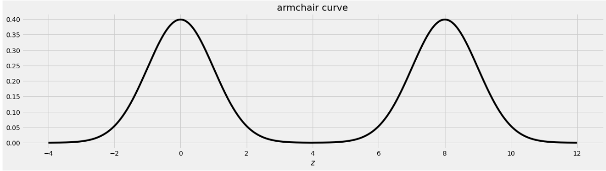
This was created by taking the portion of the standard normal distribution from z=-4 to z=4 and adjoining two copies of it, one centered at z=0 and the other centered at z=8. Let’s call this shape the armchair curve.
Since the area under the standard normal curve from z=-4 to z=4 is approximately 1, the total area under the armchair curve is approximately 2.
Complete the implementation of the two functions below:
area_left_of(z) should return the area under the
armchair curve to the left of z, assuming
-4 <= z <= 12, andarea_between(x, y) should return the area under the
armchair curve between x and y, assuming
-4 <= x <= y <= 12.import scipy
def area_left_of(z):
'''Returns the area under the armchair curve to the left of z.
Assume -4 <= z <= 12'''
if ___(a)___:
return ___(b)___
return scipy.stats.norm.cdf(z)
def area_between(x, y):
'''Returns the area under the armchair curve between x and y.
Assume -4 <= x <= y <= 12.'''
return ___(c)___What goes in blank (a)?
Answer: z>4 or
z>=4
The body of the function contains an if statement
followed by a return statement, which executes only when
the if condition is false. In that case, the function
returns scipy.stats.norm.cdf(z), which is the area under
the standard normal curve to the left of z. When
z is in the left half of the armchair curve, the area under
the armchair curve to the left of z is the area under the
standard normal curve to the left of z because the left
half of the armchair curve is a standard normal curve, centered at 0. So
we want to execute the return statement in that case, but
not if z is in the right half of the armchair curve, since
in that case the area to the left of z under the armchair
curve should be more than 1, and scipy.stats.norm.cdf(z)
can never exceed 1. This means the if condition needs to
correspond to z being in the right half of the armchair
curve, which corresponds to z>4 or z>=4,
either of which is a correct solution.
The average score on this problem was 72%.
What goes in blank (b)?
Answer:
1+scipy.stats.norm.cdf(z-8)
This blank should contain the value we want to return when
z is in the right half of the armchair curve. In this case,
the area under the armchair curve to the left of z is the
sum of two areas:
z.Since the right half of the armchair curve is just a standard normal
curve that’s been shifted to the right by 8 units, the area under that
normal curve to the left of z is the same as the area to
the left of z-8 on the standard normal curve that’s
centered at 0. Adding the portion from the left half and the right half
of the armchair curve gives
1+scipy.stats.norm.cdf(z-8).
For example, if we want to find the area under the armchair curve to the left of 9, we need to total the yellow and blue areas in the image below.
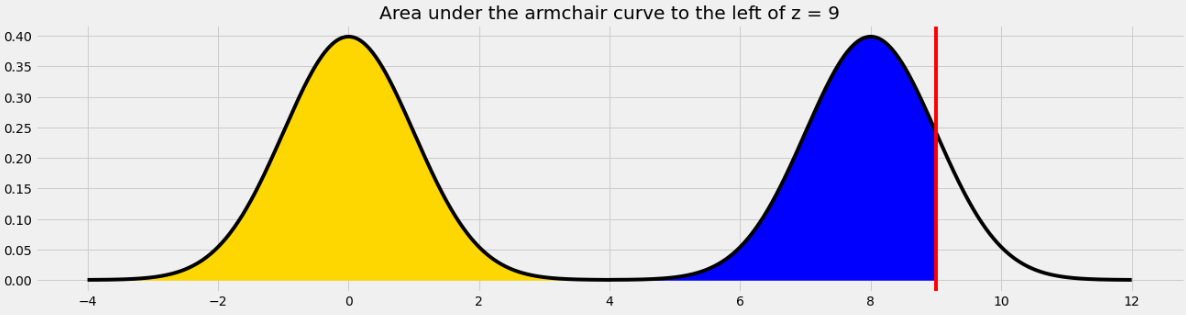
The yellow area is 1 and the blue area is the same as the area under the standard normal curve (or the left half of the armchair curve) to the left of 1 because 1 is the point on the left half of the armchair curve that corresponds to 9 on the right half. In general, we need to subtract 8 from a value on the right half to get the corresponding value on the left half.
The average score on this problem was 54%.
What goes in blank (c)?
Answer:
area_left_of(y) - area_left_of(x)
In general, we can find the area under any curve between
x and y by taking the area under the curve to
the left of y and subtracting the area under the curve to
the left of x. Since we have a function to find the area to
the left of any given point in the armchair curve, we just need to call
that function twice with the appropriate inputs and subtract the
result.
The average score on this problem was 60%.
Suppose you have correctly implemented the function
area_between(x, y) so that it returns the area under the
armchair curve between x and y, assuming the
inputs satisfy -4 <= x <= y <= 12.
Note: You can still do this question, even if you didn’t know how to do the previous one.
What is the approximate value of
area_between(-2, 10)?
1.9
1.95
1.975
2
Answer: 1.95
The area we want to find is shown below in two colors. We can find the area in each half of the armchair curve separately and add the results.
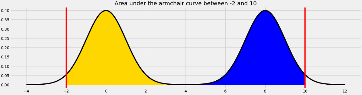
For the yellow area, we know that the area within 2 standard deviations of the mean on the standard normal curve is 0.95. The remaining 0.05 is split equally on both sides, so the yellow area is 0.975.
The blue area is the same by symmetry so the total shaded area is 0.975*2 = 1.95.
Equivalently, we can use the fact that the total area under the armchair curve is 2, and the amount of unshaded area on either side is 0.025, so the total shaded area is 2 - (0.025*2) = 1.95.
The average score on this problem was 76%.
What is the approximate value of
area_between(0.37, 8.37)?
0.68
0.95
1
1.5
Answer: 1
The area we want to find is shown below in two colors.
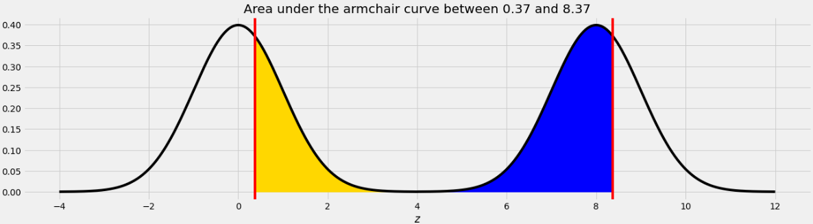
As we saw in Problem 12.2, the point on the left half of the armchair curve that corresponds to 8.37 is 0.37. This means that if we move the blue area from the right half of the armchair curve to the left half, it will fit perfectly, as shown below.
Therefore the total of the blue and yellow areas is the same as the area under one standard normal curve, which is 1.
The average score on this problem was 76%.
An IKEA employee has access to a data set of the purchase amounts for 40,000 customer transactions. This data set is roughly normally distributed with mean 150 dollars and standard deviation 25 dollars.
Why is the distribution of purchase amounts roughly normal?
because of the Central Limit Theorem
for some other reason
Answer: for some other reason
The data that we have is a sample of purchase amounts. It is not a sample mean or sample sum, so the Central Limit Theorem does not apply. The data just naturally happens to be roughly normally distributed, like human heights, for example.
The average score on this problem was 42%.
Shiv spends 300 dollars at IKEA. How would we describe Shiv’s purchase in standard units?
0 standard units
2 standard units
4 standard units
6 standard units
Answer: 6 standard units
To standardize a data value, we subtract the mean of the distribution and divide by the standard deviation:
\begin{aligned} \text{standard units} &= \frac{300 - 150}{25} \\ &= \frac{150}{25} \\ &= 6 \end{aligned}
A more intuitive way to think about standard units is the number of standard deviations above the mean (where negative means below the mean). Here, Shiv spent 150 dollars more than average. One standard deviation is 25 dollars, so 150 dollars is six standard deviations.
The average score on this problem was 97%.
Give the endpoints of the CLT-based 95% confidence interval for the mean IKEA purchase amount, based on this data.
Answer: 149.75 and 150.25 dollars
The Central Limit Theorem tells us about the distribution of the sample mean purchase amount. That’s not the distribution the employee has, but rather a distribution that shows how the mean of a different sample of 40,000 purchases might have turned out. Specifically, we know the following information about the distribution of the sample mean.
Since the distribution of the sample mean is roughly normal, we can find a 95% confidence interval for the sample mean by stepping out two standard deviations from the center, using the fact that 95% of the area of a normal distribution falls within 2 standard deviations of the mean. Therefore the endpoints of the CLT-based 95% confidence interval for the mean IKEA purchase amount are
The average score on this problem was 36%.
There are 52 IKEA locations in the United States, and there are 50 states.
Which of the following describes how to calculate the total variation distance between the distribution of IKEA locations by state and the uniform distribution?
For each IKEA location, take the absolute difference between 1/50 and the number of IKEAs in the same state divided by the total number of IKEA locations. Sum these values across all locations and divide by two.
For each IKEA location, take the absolute difference between the number of IKEAs in the same state and the average number of IKEAs in each state. Sum these values across all locations and divide by two.
For each state, take the absolute difference between 1/50 and the number of IKEAs in that state divided by the total number of IKEA locations. Sum these values across all states and divide by two.
For each state, take the absolute difference between the number of IKEAs in that state and the average number of IKEAs in each state. Sum these values across all states and divide by two.
None of the above.
Answer: For each state, take the absolute difference between 1/50 and the number of IKEAs in that state divided by the total number of IKEA locations. Sum these values across all states and divide by two.
We’re looking at the distribution across states. Since there are 50 states, the uniform distribution would correspond to having a fraction of 1/50 of the IKEA locations in each state. We can picture this as a sequence with 50 entries that are all the same: (1/50, 1/50, 1/50, 1/50, \dots)
We want to compare this to the actual distribution of IKEAs across states, which we can think of as a sequence with 50 entries, representing the 50 states, but where each entry is the proportion of IKEA locations in a given state. For example, maybe the distribution starts out like this: (3/52, 1/52, 0/52, 1/52, \dots) We can interpret each entry as the number of IKEAs in a state divided by the total number of IKEA locations. Note that this has nothing to do with the average number of IKEA locations in each state, which is 52/50.
The way we take the TVD of two distributions is to subtract the distributions, take the absolute value, sum up the values, and divide by 2. Since the entries represent states, this process aligns with the given answer.
The average score on this problem was 30%.
The HAUGA bedroom furniture set includes two items, a bed frame and a bedside table. Suppose the amount of time it takes someone to assemble the bed frame is a random quantity drawn from the probability distribution below.
| Time to assemble bed frame | Probability |
|---|---|
| 10 minutes | 0.1 |
| 20 minutes | 0.4 |
| 30 minutes | 0.5 |
Similarly, the time it takes someone to assemble the bedside table is a random quantity, independent of the time it takes them to assemble the bed frame, drawn from the probability distribution below.
| Time to assemble bedside table | Probability |
|---|---|
| 30 minutes | 0.3 |
| 40 minutes | 0.4 |
| 50 minutes | 0.3 |
What is the probability that Stella assembles the bed frame in 10 minutes if we know it took her less than 30 minutes to assemble? Give your answer as a decimal between 0 and 1.
Answer: 0.2
We want to find the probability that Stella assembles the bed frame in 10 minutes, given that she assembles it in less than 30 minutes. The multiplication rule can be rearranged to find the conditional probability of one event given another.
\begin{aligned} P(A \text{ and } B) &= P(A \text{ given } B)*P(B)\\ P(A \text{ given } B) &= \frac{P(A \text{ and } B)}{P(B)} \end{aligned}
Let’s, therefore, define events A and B as follows:
Since 10 minutes is less than 30 minutes, A \text{ and } B is the same as A in this case. Therefore, P(A \text{ and } B) = P(A) = 0.1.
Since there are only two ways to complete the bed frame in less than 30 minutes (10 minutes or 20 minutes), it is straightforward to find P(B) using the addition rule P(B) = 0.1 + 0.4. The addition rule can be used here because assembling the bed frame in 10 minutes and assembling the bed frame in 20 minutes are mutually exclusive. We could alternatively find P(B) using the complement rule, since the only way not to complete the bed frame in less than 30 minutes is to complete it in exactly 30 minutes, which happens with a probability of 0.5. We’d get the same answer, P(B) = 1 - 0.5 = 0.5.
Plugging these numbers in gives our answer.
\begin{aligned} P(A \text{ given } B) &= \frac{P(A \text{ and } B)}{P(B)}\\ &= \frac{0.1}{0.5}\\ &= 0.2 \end{aligned}
The average score on this problem was 72%.
What is the probability that Ryland assembles the bedside table in 40 minutes if we know that it took him 30 minutes to assemble the bed frame? Give your answer as a decimal between 0 and 1
Answer: 0.4
We are told that the time it takes someone to assemble the bedside table is a random quantity, independent of the time it takes them to assemble the bed frame. Therefore we can disregard the information about the time it took him to assemble the bed frame and read directly from the probability distribution that his probability of assembling the bedside table in 40 minutes is 0.4.
The average score on this problem was 82%.
What is the probability that Jin assembles the complete HAUGA set in at most 60 minutes? Give your answer as a decimal between 0 and 1.
Answer: 0.53
There are several different ways for the total assembly time to take at most 60 minutes:
Using the multiplication rule, these probabilities are:
Finally, adding them up because they represent mutually exclusive cases, we get 0.1+0.28+0.15 = 0.53.
The average score on this problem was 58%.
Suppose the price of an IKEA product and the cost to have it assembled are linearly associated with a correlation of 0.8. Product prices have a mean of 140 dollars and a standard deviation of 40 dollars. Assembly costs have a mean of 80 dollars and a standard deviation of 10 dollars. We want to predict the assembly cost of a product based on its price using linear regression.
The NORDMELA 4-drawer dresser sells for 200 dollars. How much do we predict its assembly cost to be?
Answer: 92 dollars
We first use the formulas for the slope, m, and intercept, b, of the regression line to find the equation. For our application, x is the price and y is the assembly cost since we want to predict the assembly cost based on price.
\begin{aligned} m &= r*\frac{\text{SD of }y}{\text{SD of }x} \\ &= 0.8*\frac{10}{40} \\ &= 0.2\\ b &= \text{mean of }y - m*\text{mean of }x \\ &= 80 - 0.2*140 \\ &= 80 - 28 \\ &= 52 \end{aligned}
Now we know the formula of the regression line and we simply plug in x=200 to find the associated y value.
\begin{aligned} y &= mx+b \\ y &= 0.2x+52 \\ &= 0.2*200+52 \\ &= 92 \end{aligned}
The average score on this problem was 76%.
The IDANÄS wardrobe sells for 80 dollars more than the KLIPPAN loveseat, so we expect the IDANÄS wardrobe will have a greater assembly cost than the KLIPPAN loveseat. How much do we predict the difference in assembly costs to be?
Answer: 16 dollars
The slope of a line describes the change in y for each change of 1 in x. The difference in x values for these two products is 80, so the difference in y values is m*80 = 0.2*80 = 16 dollars.
An equivalent way to state this is:
\begin{aligned} m &= \frac{\text{ rise, or change in } y}{\text{ run, or change in } x} \\ 0.2 &= \frac{\text{ rise, or change in } y}{80} \\ 0.2*80 &= \text{ rise, or change in } y \\ 16 &= \text{ rise, or change in } y \end{aligned}
The average score on this problem was 65%.
If we create a 95% prediction interval for the assembly cost of a 100 dollar product and another 95% prediction interval for the assembly cost of a 120 dollar product, which prediction interval will be wider?
The one for the 100 dollar product.
The one for the 120 dollar product.
Answer: The one for the 100 dollar product.
Prediction intervals get wider the further we get from the point (\text{mean of } x, \text{mean of } y) since all regression lines must go through this point. Since the average product price is 140 dollars, the prediction interval will be wider for the 100 dollar product, since it’s the further of 100 and 120 from 140.
The average score on this problem was 45%.
For each IKEA desk, we know the cost of producing the desk, in dollars, and the current sale price of the desk, in dollars. We want to predict sale price based on production cost using linear regression.
For this scenario, which of the following most likely describes the slope of the regression line when both variables are measured in dollars?
less than 0
between 0 and 1, exclusive
more than 1
none of the above (exactly equal to 0 or 1)
Answer: more than 1
The slope of a line represents the change in y for each change of 1 in x. Therefore, the slope of the regression line is the amount we’d predict the sale price to increase when the production cost of an item increases by one dollar. In other words, it’s the sale price per dollar of production cost. This is almost certainly more than 1, otherwise the company would not make a profit. We’d expect that for any company, the sale price of an item should exceed the production cost, meaning the slope of the regression line has a value greater than one.
The average score on this problem was 72%.
For this scenario, which of the following most likely describes the slope of the regression line when both variables are measured in standard units?
less than 0
between 0 and 1, exclusive
more than 1
none of the above (exactly equal to 0 or 1)
Answer: between 0 and 1, exclusive
When both variables are measured in standard units, the slope of the regression line is the correlation coefficient. Recall that correlation coefficients are always between -1 and 1, however, because it’s not realistic for production cost and sale price to be negatively correlated (as that would mean products sell for less if they cost more to produce) we can limit our choice of answer to values between 0 and 1. Because a coefficient of 0 would mean there is no correlation and 1 would mean perfect correlation (that is, plotting the data would create a line), these are unlikely occurrences leaving us with the answer being between 0 and 1, exclusive.
The average score on this problem was 86%.
The residual plot for this regression is shown below.
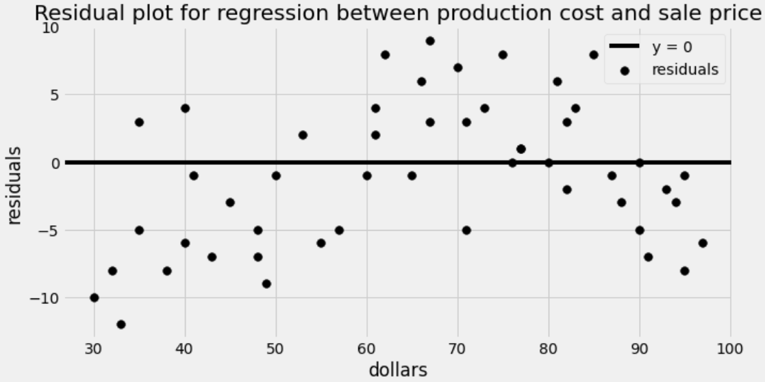
What is being represented on the horizontal axis of the residual plot?
actual production cost
actual sale price
predicted production cost
predicted sale price
Answer: actual production cost
Residual plots show x on the horizontal axis and the residuals, or differences between actual y values and predicted y values, on the vertical axis. Therefore, the horizontal axis here shows the production cost. Note that we are not predicting production costs at all, so production cost means the actual cost to produce a product.
The average score on this problem was 43%.
Which of the following is a correct conclusion based on this residual plot? Select all that apply.
The correlation between production cost and sale price is weak.
It would be better to fit a nonlinear curve.
Our predictions will be more accurate for some inputs than others.
We don’t have enough data to do regression.
The regression line is not the best-fitting line for this data set.
The data set is not representative of the population.
Answer: It would be better to fit a nonlinear curve.
Let’s go through each answer choice.
The correlation between production cost and sale price could be very strong. After all, we are able to predict the sale price within ten dollars almost all the time, since residuals are almost all between -10 and 10.
It would be better to fit a nonlinear curve because the residuals show a pattern. Reading from left to right, they go from mostly negative to mostly positive to mostly negative again. This suggests that a nonlinear curve might be a better fit for our data.
Our predictions are typically within ten dollars of the actual sale price, and this is consistent throughout. We see this on the residual plot by a fairly even vertical spread of dots as we scan from left to right. This data is not heteroscedastic.
We can do regression on a dataset of any size, even a very small data set. Further, this dataset is decently large, since there are a good number of points in the residual plot.
The regression line is always the best-fitting line for any dataset. There may be other curves that are better fits than lines, but when we restrict to lines, the best of the bunch is the regression line.
We have no way of knowing how representative our data set is of the population. This is not something we can discern from a residual plot because such a plot contains no information about the population from which the data was drawn.
The average score on this problem was 61%.