← return to practice.dsc10.com
Instructor(s): Suraj Rampure
This exam was administered in-person. The exam was closed-notes, except students were provided a copy of the DSC 10 Reference Sheet. No calculators were allowed. Students had 3 hours to take this exam.
Note (groupby / pandas 2.0): Pandas 2.0+ no longer
silently drops columns that can’t be aggregated after a
groupby, so code written for older pandas may behave
differently or raise errors. In these practice materials we use
.get() to select the column(s) we want after
.groupby(...).mean() (or other aggregations) so that our
solutions run on current pandas. On real exams you will not be penalized
for omitting .get() when the old behavior would have
produced the same answer.
Here’s a walkthrough video of Problems 3, 5, and 6, and here’s a walkthrough video of Problems 7, 8.4, 10, and 11.
You may have noticed that San Diego was quite cloudy in May (2023). In fact, according to the National Weather Service, San Diego was the single cloudiest city in the contiguous United States in May, with clouds covering the sky 82% of the time. (Only a remote town in Alaska was cloudier!)
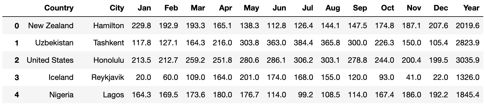
In this exam, we will work with the DataFrame sun, which
describes the number of sunshine hours per month in various cities
around the world. Each number in sun is an average across
multiple years and multiple sensors.
The first 2 columns in sun are "Country"
and "City", which are strings describing a particular city.
The next 12 columns are "Jan", "Feb",
"Mar", …, "Dec", which describe the number of
sunshine hours seen each month. The last column, "Year", is
the sum of the month-specific columns.
The first few rows of sun are shown below, though
sun has many more rows than are shown below.
For instance, we see that Tashkent, Uzbekistan sees 164.3 sunshine hours in March.
Throughout the exam, assume that we have already run
import babypandas as bpd and
import numpy as np.
Complete the implementation of the function
most_sunshine, which takes in country, the
name of a country, and month, the name of a month
(e.g. "Apr"), and returns the name of the city (as a
string) in country with the most sunshine hours in
month, among the cities in sun. Assume there
are no ties.
    def most_sunshine(country, month):
        country_only = __(a)__
        return country_only.__(b)__
What goes in blanks (a) and (b)?
Answer: (a):
sun[sun.get("Country") == country], (b):
sort_values(month).get("City").iloc[-1] or
sort_values(month, ascending=False).get("City").iloc[0]
What goes in blank (a)?
sun[sun.get("Country") == country] To identify cities only
within the specified country, we need to query for the rows in the
sun DataFrame where the "Country" column
matches the given country. The expression
sun.get("Country") == country creates a Boolean Series,
where each entry is True if the corresponding row’s
"Country" column matches the provided country
and False otherwise. When this Boolean series is used to
index into sun DataFrame, it keeps only the rows for which
sun.get("Country") == country is True,
effectively giving us only the cities from the specified country.
The average score on this problem was 78%.
What goes in blank (b)?
sort_values(month).get("City").iloc[-1] or
sort_values(month, ascending=False).get("City").iloc[0]
To determine the city with the most sunshine hours in the specified
month, we sort the queried DataFrame (which only contains cities from
the specified country) based on the values in the month
column. There are two ways to achieve the desired result:
.iloc[-1] to get the last item after selecting the
"City" column with .get("City")..iloc[0] to get the
first item after selecting the "City" column with
.get("City").Both methods will give us the name of the city with the most sunshine hours in the specified month.
The average score on this problem was 52%.
In this part only, assume that all "City" names in
sun are unique.
Consider the DataFrame cities defined below.
cities = sun.groupby("City").mean().reset_index()Fill in the blanks so that the DataFrame that results from the
sequence of steps described below is identical to
cities.
“Sort sun by (c) in
(d) order (e).”
What goes in blank (c)?
"Country"
"City"
"Jan"
"Year"
What goes in blank (d)?
ascending
descending
What goes in blank (e)?
and drop the "Country" column
and drop the "Country" and "City"
columns
and reset the index
, drop the "Country" column, and reset the index
, drop the "Country" and "City" columns,
and reset the index
Nothing, leave blank (e) empty
Answer: (c): "City", (d): ascending,
(e): drop the "Country" column, and reset the index
Let’s start by understanding the code provided in the question:
The .groupby("City") method groups the data in the
sun DataFrame by unique city names. Since every city name
in the DataFrame is unique, this means that each group will consist of
just one row corresponding to that city.
After grouping by city, the .mean() method computes the
average of each column for each group. Again, as each city name is
unique, this operation doesn’t aggregate multiple rows but merely
reproduces the original values for each city. (For example, the value in
the "Jan" column for the row with the index
"Hamilton" will just be 229.8, which we see in the first
row of the preview of sun.)
Finally, .reset_index() is used to reset the DataFrame’s
index. When using .groupby, the column we group by (in this
case, "City") becomes the index. By resetting the index,
we’re making "City" a regular column again and setting the
index to 0, 1, 2, 3, …
What goes in blank (c)? "City"
When we group on "City", the index of the DataFrame is set
to "City" names, sorted in ascending alphabetical order
(this is always the behavior of groupby). Since all city
names are unique, the number of rows in
sun.groupby("City").mean() is the same as the number of
rows in sun, and so grouping on "City"
effectively sorts the DataFrame by "City" and sets the
index to "City". To replicate the order in
cities, then, we must sort sun by the
"City" column in ascending order.
The average score on this problem was 97%.
What goes in blank (d)? ascending
Addressed above.
The average score on this problem was 77%.
What goes in blank (e)? , drop the
"Country" column, and reset the index
In the provided code, after grouping by "City" and
computing the mean, we reset the index. This means the
"City" column is no longer the index but a regular column,
and the DataFrame gets a fresh integer index. To replicate this
structure, we need to reset the index in our sorted DataFrame.
Additionally, when we applied the .mean() method after
grouping, any non-numeric columns (like "Country") that we
can’t take the mean of are automatically excluded from the resulting
DataFrame. To match the structure of cities, then, we must
drop the "Country" column from our sorted DataFrame.
The average score on this problem was 46%.
True or False: In the code below, Z is guaranteed to
evaluate to True.
x = sun.groupby(["Country", "Year"]).mean().shape[0]
y = sun.groupby("Country").mean().shape[0]
z = (x >= y)
True
False
Answer: True
Let’s us look at each line of code separately:
x = sun.groupby(["Country", "Year"]).mean().shape[0]:
This line groups the sun DataFrame by both
"Country" and "Year", then computes the mean.
As a result, each unique combination of "Country" and
"Year" will have its own row. For instance, if there are
three different values in the "Year" column for a
particular country, that country will appear three times in the
DataFrame sun.groupby(["Country", "Year"]).mean().
y = sun.groupby("Country").mean().shape[0]: When
grouping by "Country" alone, each unique country in the
sun DataFrame is represented by one row, independent of the
information in other columns.
z = (x >= y): This comparison checks whether the
number of rows produced by grouping by both "Country" and
"Year" (which is x) is greater than or equal
to the number of rows produced by grouping only by
"Country" (which is y).
Given our grouping logic:
If every country in the sun DataFrame has only a
single unique value in the "Year" column (e.g. if the
"Year" value for all ciites in the United States was always
3035.9, and if the "Year" value for all cities in Nigeria
was always 1845.4, etc.), then the number of rows when grouping by both
"Country" and "Year" will be equal to the
number of rows when grouping by "Country" alone. In this
scenario, x will be equal to y.
If at least one country in the sun DataFrame has at
least two different values in the "Year" column (e.g. if
there are at least two cities in the United States with different values
in the "Year" column), then there will be more rows when
grouping by both "Country" and "Year" compared
to grouping by "Country" alone. This means x
will be greater than y.
Considering the above scenarios, there’s no situation where the value
of x can be less than the value of y.
Therefore, z will always evaluate to True.
The average score on this problem was 70%.
In the next few parts, consider the following answer choices.
The name of the country with the most cities.
The name of the country with the fewest cities.
The number of cities in the country with the most cities.
The number of cities in the country with the fewest cities.
The last city, alphabetically, in the first country, alphabetically.
The first city, alphabetically, in the first country, alphabetically.
Nothing, because it errors.
What does the following expression evaluate to?
sun.groupby("Country").max().get("City").iloc[0]A
B
C
D
E
F
G
Answer: E. The last city, alphabetically, in the
first country, alphabetically.
Let’s break down the code:
sun.groupby("Country").max(): This line of code
groups the sun DataFrame by the "Country"
column and then determines the maximum for every other
column within each country group. Since the values in the
"City" column are stored as strings, and the maximum of a
Series of strings is the last string alphabetically, the values in the
"City" column of this DataFrame will contain the last city,
alphabetically, of each country.
.get("City"): .get("City") accesses the
"City" column.
.iloc[0]: Finally, .iloc[0] selects the
"City" value from the first row. The first row corresponds
to the first country alphabetically because groupby sorted
the DataFrame by "Country" in ascending order. The value in
the "City" column that .iloc[0] selects, then,
is the name of the last city, alphabetically, in the first country,
alphabetically.
The average score on this problem was 36%.
What does the following expression evaluate to?
sun.groupby("Country").sum().get("City").iloc[0]A
B
C
D
E
F
G
Answer: G. Nothing, because it errors.
Let’s break down the code:
sun.groupby("Country").sum(): This groups the
sun DataFrame by the "Country" column and
computes the sum for each numeric column within each country group.
Since "City" is non-numeric, it will be dropped.
.get("City"): This operation attempts to retrieve
the "City" column from the resulting DataFrame. However,
since the "City" column was dropped in the previous step,
this will raise a KeyError, indicating that the column is not present in
the DataFrame.
The average score on this problem was 73%.
What does the following expression evaluate to?
sun.groupby("Country").count().sort_values("Jan").index[-1]A
B
C
D
E
F
G
Answer: A. The name of the country with the most
cities.
Let’s break down the code:
sun.groupby("Country").count(): This groups the sun
DataFrame by the "Country" column. The
.count() method then returns the number of rows in each
group for each column. Since we’re grouping by "Country",
and since the rows in sun correspond to cities, this is
counting the number of cities in each country.
.sort_values("Jan"): The result of the previous
operation is a DataFrame with "Country" as the index and
the number of cities per country stored in every other column. The
"City, "Jan", "Feb",
"Mar", etc. columns in the resulting DataFrame all contain
the same information. Sorting by "Jan" sorts the DataFrame
by the number of cities each country has in ascending order.
.index[-1]: This retrieves the last index value from
the sorted DataFrame, which corresponds to the name of the country with
the most cities.
The average score on this problem was 61%.
What does the following expression evaluate to?
sun.groupby("Country").count().sort_values("City").get("City").iloc[-1]A
B
C
D
E
F
G
Answer: C. The number of cities in the country with
the most cities.
Let’s break down the code:
sun.groupby("Country").count(): This groups the sun
DataFrame by the "Country" column. The
.count() method then returns the number of rows in each
group for each column. Since we’re grouping by "Country",
and since the rows in sun correspond to cities, this is
counting the number of cities in each country.
.sort_values("City"): The result of the previous
operation is a DataFrame with "Country" as the index and
the number of "City"s per "Country" stored in
every other column. The "City, "Jan",
"Feb", "Mar", etc. columns in the resulting
DataFrame all contain the same information. Sorting by
"City" sorts the DataFrame by the number of cities each
country has in ascending order.
.get("City"): This retrieves the "City"
column from the sorted DataFrame, which contains the number of cities in
each country.
.iloc[-1]: This gets the last value from the
"City" column, which corresponds to the number of cities in
the country with the most cities.
The average score on this problem was 57%.
Vanessa is a big Formula 1 racing fan, and wants to plan a trip to Monaco, where the Monaco Grand Prix is held. Monaco is an example of a “city-state” — that is, a city that is its own country. Singapore is another example of a city-state.
We’ll say that a row of sun corresponds to a city-state
if its "Country" and "City" values are
equal.
Fill in the blanks so that the expression below is equal to the total
number of sunshine hours in October of all city-states in
sun.
sun[__(a)__].__(b)__What goes in blanks (a) and (b)?
Answer: (a):
sun.get("Country") == sun.get("City"), (b):
.get("Oct").sum()
What goes in blank (a)?
sun.get("Country") == sun.get("City")
This expression compares the "Country" column to the
"City" column for each row in the sun
DataFrame. It returns a Boolean Series where each value is
True if the corresponding "Country" and
"City" are the same (indicating a city-state) and
False otherwise.
The average score on this problem was 79%.
What goes in blank (b)?
.get("Oct").sum()
Here, we select the "Oct" column, which represents the
sunshine hours in October, and compute the sum of its values. By using
this after querying for city-states, we calculate the total sunshine
hours in October across all city-states in the sun
DataFrame.
The average score on this problem was 85%.
Fill in the blanks below so that the expression below is also equal
to the total number of sunshine hours in October of all city-states in
sun.
Note: What goes in blank (b) is the same as what goes in blank (b) above.
sun.get(["Country"]).merge(__(c)__).__(b)__What goes in blank (c)?
Answer:
sun, left_on="Country", right_on="City"
Let’s break down the code:
sun.get(["Country"]): This extracts just the
"Country" column from the sun DataFrame, as a
DataFrame. (It’s extracted as a DataFrame since we passed a list to
.get instead of a single string.)
.merge(sun, left_on="Country", right_on="City"):
Here, we’re using the .merge method to merge a version of
sun with just the "Country" column (which is
our left DataFrame) with the entire sun DataFrame
(which is our right DataFrame). The merge is done by matching
"Country"s from the left DataFrame with
"City"s from the right DataFrame. This way, rows in the
resulting DataFrame correspond to city-states, as it only contains
entries where a country’s name is the same as a city’s name.
.get("Oct").sum(): After merging, we use
.get("Oct") to retrieve the "Oct" column,
which represents the sunshine hours in October. Finally,
.sum() computes the total number of sunshine hours in
October for all the identified city-states.
The average score on this problem was 50%.
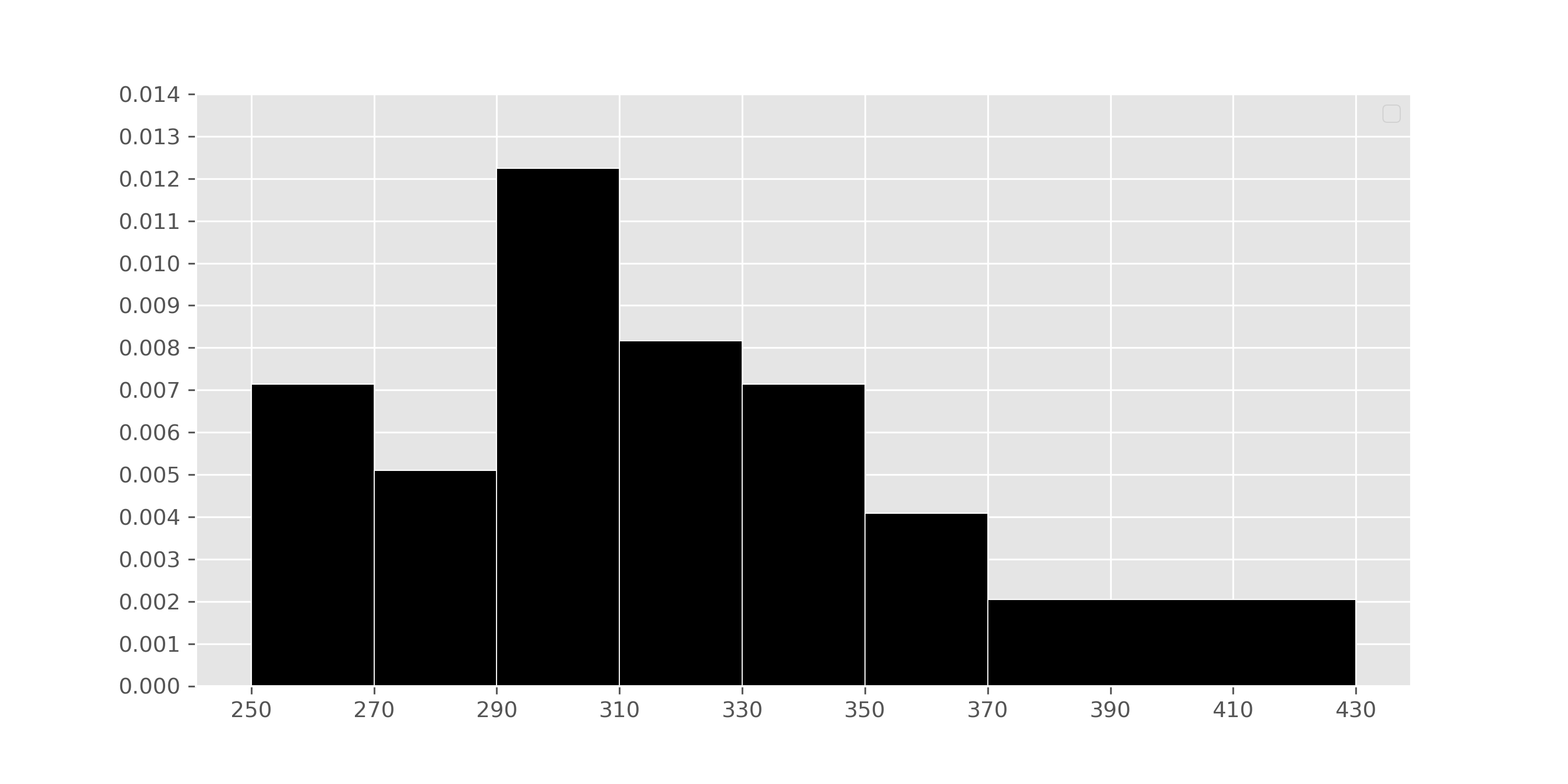
This summer, Zoe wants to explore parts of the United States that she
hasn’t been to yet. In her process of figuring out where to go, she
creates a histogram depicting the distribution of the number of sunshine
hours in July across all cities in the United States in
sun.
Suppose usa is a DataFrame with all of the columns in
sun but with only the rows where "Country" is
"United States".
What is the value of mystery below?
    cond = (usa.get("Jul") >= 370) & (usa.get("Jul") < 430)
    mystery = 100 * np.count_nonzero(cond) / usa.shape[0]
2
8
12
16
18
20
Answer: 12
cond is a Series that contains True for
each row in usa where "Jul" is greater than or
equal to 370 and less than 430. mystery, then, is the
percentage of values in usa in which
cond is True. This is because
np.count_nonzero(cond) is the number of Trues
in cond, np.count_nonzero(cond) / usa.shape[0]
is the proportion of values in cond that are
True, and
100 * np.count_nonzero(cond) / usa.shape[0] is the
percentage of values in cond that are True.
Our goal here, then, is to use the histogram to find the
percentage of values in the histogram between 370 (inclusive) and 430
(exclusive).
We know that in histograms, the area of each bar is equal to the proportion of data points that fall within its bin’s range. Conveniently, there’s only one bar we need to look at – the one corresponding to the bin [370, 430). That bar has a width of 430 - 370 = 60 and a height of 0.002. Then, the area of that bar – i.e. the proportion of values that are between 370 (inclusive) and 430 (exclusive) is:
\text{proportion} = \text{area} = \text{height} \cdot \text{width} = 0.002 \cdot 60 = 0.12
This means that the proportion of values in [370, 430) is 0.12, which
means that the percentage of values in [370, 430) is 12%, and that
mystery evaluates to 12.
The average score on this problem was 83%.
There are 5 more cities with between 370 and 430 sunshine hours in July than there are cities with between 270 and 290 sunshine hours in July.
How many cities in the United States are in sun? Give
your answer as a positive integer, rounded to the nearest multiple of 10
(that is, your answer should end in a 0).
Answer: 250
In the previous part, we learned that the proportion of cities in the
usa DataFrame in the interval [370, 430) (i.e. that have
between 370 and 430 sunshine hours in July) is 0.12. To use the fact
that there are 5 more cities in the interval [370, 430) than there are
in the interval [270, 290), we need to first find the proportion of
cities in the interval [270, 290). To do so, we look at the [270, 290)
bin, which has a width of 290 - 270 =
20 and a height of 0.005:
\text{proportion} = 0.005 \cdot 20 = 0.10
We are told that there are 5 more cities in the [370, 430) interval than there are in the [270, 290) interval. Given the proportions we’ve computed, we have that:
\text{difference in proportions} = 0.12 - 0.1 = 0.02
If 0.02 \cdot \text{number of cities} is 5, then \text{number of cities} = 5 \cdot \frac{1}{0.02} = 5 \cdot 50 = 250.
The average score on this problem was 49%.
Now, suppose we convert the number of sunshine hours in July for all
cities in the United States (i.e., “US cities”) in sun from
their original units (hours) to standard units.
Let m be the mean number of sunshine
hours in July for all US cities in sun, in standard units.
Select the true statement below.
m = -1
-1 < m < 0
m = 0
0 < m < 1
m = 1
m > 1
Answer: m = 0
When we standardize a dataset, the mean of the resulting values is always 0 and the standard deviation of the resulting values is always 1. This tells us right away that the answer is m = 0. Intuitively, we know that a value in standard units represents the number of standard deviations that value is above or below the mean of the column it came from. m is equal to the mean of the column it came from, so m in standard units is 0.
If we’d like to approach this more algebracically, we can remember the formula for converting a value x_i from a column x to standard units:
x_{i \: \text{(su)}} = \frac{x_i - \text{mean of } x}{\text{SD of } x}
Let x be the column (i.e. Series)
containing the mean number of sunshine hours in July for all US cities
in sun. m, by definition,
is the mean of x. Then,
m_{\text{(su)}} = \frac{m - \text{mean of } x}{\text{SD of } x} = \frac{m - m}{\text{SD of }x} = 0
Given that m is the mean of column x, the numerator of m_\text{(su)} is 0, and hence m_\text{(su)} is 0.
The average score on this problem was 62%.
Let s be the standard deviation of
the number of sunshine hours in July for all US cities sun,
in standard units. Select the true statement below.
s = -1
-1 < s <0
s = 0
0 < s < 1
s = 1
s > 1
Answer: s = 1
As mentioned in the previous solution, when we standardize a dataset, the mean of the resulting values is always 0 and the standard deviation of the resulting values is always 1.
The average score on this problem was 46%.
Let d be the median of the number of
sunshine hours in July for all US cities in sun, in
standard units. Select the true statement below.
d = -1
-1 < d < 0
d = 0
0 < d < 1
d = 1
d > 1
Answer: -1 < d <
0
In the histogram, we see that the distribution of the number of
sunshine hours in July for all US cities in sunis skewed
right, or has a right tail. This means that this distribution’s mean is
dragged in the direction of its tail and is larger than its median.
Since the mean in standard units is 0, and the median is less than the
mean, the median in standard units must be negative. There’s no property
that states that the median is exactly -1, and the median is only
slightly less than the mean, which means that it must be the case that
-1 < d < 0.
The average score on this problem was 42%.
True or False: The distribution of the number of sunshine hours in
July for all US cities in sun, in standard units, is
roughly normal.
True
False
Impossible to tell
Answer: False
The original histogram depicting the distribution of the number of sunshine hours in July for all US cities is right-skewed. When data is converted to standard units, the shape of the distribution does not change. Therefore, if the original data is right-skewed, the standardized data will also be right-skewed.
The average score on this problem was 45%.
For each city in sun, we have 12 numbers, corresponding
to the number of sunshine hours it sees in January, February, March, and
so on, through December. (There is also technically a 13th number, the
value in the "Year" column, but we will ignore it for the
purposes of this question.)
We say that a city’s number of sunshine hours peaks gradually if both of the following conditions are true:
Each month from February to June has a number of sunshine hours greater than or equal to the month before it.
Each month from August to December has a number of sunshine hours less than or equal to the month before it.
For example, the number of sunshine hours per month in Doris’ hometown of Guangzhou, China peaks gradually:
62, 65, 71, 104, 118, 202, 181, 173, 172, 170, 166, 140
However, the number of sunshine hours per month in Charlie’s hometown of Redwood City, California does not peak gradually, since 325 > 311 and 247 < 271:
185, 207, 269, 309, 325, 311, 313, 287, 247, 271, 173, 160
Complete the implementation of the function
peaks_gradually, which takes in an array hours
of length 12 corresponding to the number of sunshine hours per month in
a city, and returns True if the city’s number of sunshine
hours peaks gradually and False otherwise.
    def peaks_gradually(hours):
        for i in np.arange(5):
            cur_left = hours[5 - i]
            next_left = hours[__(a)__]
            cur_right = hours[__(b)__]
            next_right = hours[6 + i + 1]

            if __(c)__:
                __(d)__

__(e)__What goes in blank (a)?
Answer: 5 - i - 1 or
4 - i
Before filling in the blanks, let’s discuss the overall strategy of the problem. The idea is as follows
cur_left, which is the sunshine hours for June
(month 5, since 5 - i = 5 - 0 = 5), to
next_left, which is the sunshine hours for May (month 5 - i - 1 = 4). If
next_left > cur_left, it means that May has more
sunshine hours than June, which means the sunshine hours for this city
don’t peak gradually. (Remember, for the number of sunshine hours to
peak gradually, we need it to be the case that each month from February
to June has a number of sunshine hours greater than or equal to the
month before it.)cur_right, which is the sunshine hours
for July (month 6, since 6 + i = 6 + 0 =
6), to next_right, which is the sunshine hours for
August (month 6 + i + 1 = 7). If
next_right > cur_right, it means that August has more
sunshine hours than July, which means the sunshine hours for this city
don’t peak gradually. (Remember, for the number of sunshine hours to
peak gradually, we need it to be the case that each month from August to
December has a number of sunshine hours less than or equal to the month
before it.)next_left > cur_left or next_right > cur_right, then
we don’t need to look at any other pairs of months, and can just
return False. Otherwise, we keep looking.cur_left
and next_left will “step backwards” and refer to May (month
4, since 5 - i = 5 - 1 = 4) and April
(month 3, since 5 - i - 1 = 3),
respectively. Simililarly, cur_right and
next_right will “step forwards” and refer to August and
September, respectively. The above process is repeated.next_left > cur_left or next_right > cur_right was
never True, then it must be the case that the sunshine
hours for this city peak gradually, and we can return True
outside of the for-loop!Focusing on blank (a) specifically, it needs to contain the position
of next_left, which is the index of the month before the
current left month. Since the current month is at 5 - i,
the next month needs to be at 5 - i - 1.
The average score on this problem was 62%.
What goes in blank (b)?
Answer: 6 + i
Using the same logic as for blank (a), blank (b) needs to contain the
position of cur_right, which is the index of the month
before the next right month. Since the next right month is at
6 + i + 1, the current right month is at
6 + i.
The average score on this problem was 67%.
What goes in blank (c)?
next_left < cur_left or next_right < cur_right
next_left < cur_left and next_right < cur_right
next_left > cur_left or next_right > cur_right
next_left > cur_left and next_right > cur_right
Answer:
next_left > cur_left or next_right > cur_right
Explained in the answer to blank (a).
The average score on this problem was 35%.
What goes in blank (d)?
return True
return False
Answer: return False
Explained in the answer to blank (a).
The average score on this problem was 50%.
What goes in blank (e)?
return True
return False
Answer: return True
Explained in the answer to blank (a).
The average score on this problem was 54%.
In some cities, the number of sunshine hours per month is relatively consistent throughout the year. São Paulo, Brazil is one such city; in all months of the year, the number of sunshine hours per month is somewhere between 139 and 173. New York City’s, on the other hand, ranges from 139 to 268.
Gina and Abel, both San Diego natives, are interested in assessing how “consistent" the number of sunshine hours per month in San Diego appear to be. Specifically, they’d like to test the following hypotheses:
Null Hypothesis: The number of sunshine hours per month in San Diego is drawn from the uniform distribution, \left[\frac{1}{12}, \frac{1}{12}, ..., \frac{1}{12}\right]. (In other words, the number of sunshine hours per month in San Diego is equal in all 12 months of the year.)
Alternative Hypothesis: The number of sunshine hours per month in San Diego is not drawn from the uniform distribution.
As their test statistic, Gina and Abel choose the total variation distance. To simulate samples under the null, they will sample from a categorical distribution with 12 categories — January, February, and so on, through December — each of which have an equal probability of being chosen.
In order to run their hypothesis test, Gina and Abel need a way to calculate their test statistic. Below is an incomplete implementation of a function that computes the TVD between two arrays of length 12, each of which represent a categorical distribution.
    def calculate_tvd(dist1, dist2):
        return np.mean(np.abs(dist1 - dist2)) * ____
Fill in the blank so that calculate_tvd works as
intended.
1 / 6
1 / 3
1 / 2
2
3
6
Answer: 6
The TVD is the sum of the absolute differences in proportions,
divided by 2. In the code to the left of the blank, we’ve computed the
mean of the absolute differences in proportions, which is the same as
the sum of the absolute differences in proportions, divided by 12 (since
len(dist1) is 12). To correct the fact that we
divided by 12, we multiply by 6, so that we’re only dividing by 2.
The average score on this problem was 17%.
Moving forward, assume that calculate_tvd works
correctly.
Now, complete the implementation of the function
uniform_test, which takes in an array
observed_counts of length 12 containing the number of
sunshine hours each month in a city and returns the p-value for the
hypothesis test stated at the start of the question.
    def uniform_test(observed_counts):
        # The values in observed_counts are counts, not proportions!
        total_count = observed_counts.sum()
        uniform_dist = __(b)__
        tvds = np.array([])
        for i in np.arange(10000):
            simulated = __(c)__
            tvd = calculate_tvd(simulated, __(d)__)
            tvds = np.append(tvds, tvd)
return np.mean(tvds __(e)__ calculate_tvd(uniform_dist, __(f)__))What goes in blank (b)? (Hint: The function
np.ones(k) returns an array of length k in
which all elements are 1.)
Answer: np.ones(12) / 12
uniform_dist needs to be the same as the uniform
distribution provided in the null hypothesis, \left[\frac{1}{12}, \frac{1}{12}, ...,
\frac{1}{12}\right].
In code, this is an array of length 12 in which each element is equal
to 1 / 12. np.ones(12)
creates an array of length 12 in which each value is 1; for
each value to be 1 / 12, we divide np.ones(12)
by 12.
The average score on this problem was 66%.
What goes in blank (c)?
np.random.multinomial(12, uniform_dist)
np.random.multinomial(12, uniform_dist) / 12
np.random.multinomial(12, uniform_dist) / total_count
np.random.multinomial(total_count, uniform_dist)
np.random.multinomial(total_count, uniform_dist) / 12
np.random.multinomial(total_count, uniform_dist) / total_count
Answer:
np.random.multinomial(total_count, uniform_dist) / total_count
The idea here is to repeatedly generate an array of proportions that
results from distributing total_count hours across the 12
months in a way that each month is equally likely to be chosen. Each
time we generate such an array, we’ll determine its TVD from the uniform
distribution; doing this repeatedly gives us an empirical distribution
of the TVD under the assumption the null hypothesis is true.
The average score on this problem was 21%.
What goes in blank (d)?
Answer: uniform_dist
As mentioned above:
Each time we generate such an array, we’ll determine its TVD from the uniform distribution; doing this repeatedly gives us an empirical distribution of the TVD under the assumption the null hypothesis is true.
The average score on this problem was 54%.
What goes in blank (e)?
>
>=
<
<=
==
!=
Answer: >=
The purpose of the last line of code is to compute the p-value for the hypothesis test. Recall, the p-value of a hypothesis test is the proportion of simulated test statistics that are as or more extreme than the observed test statistic, under the assumption the null hypothesis is true. In this context, “as extreme or more extreme” means the simulated TVD is greater than or equal to the observed TVD (since larger TVDs mean “more different”).
The average score on this problem was 77%.
What goes in blank (f)?
Answer: observed_counts / total_count
or observed_counts / observed_counts.sum()
Blank (f) needs to contain the observed distribution of sunshine hours (as an array of proportions) that we compare against the uniform distribution to calculate the observed TVD. This observed TVD is then compared with the distribution of simulated TVDs to calculate the p-value. The observed counts are converted to proportions by dividing by the total count so that the observed distribution is on the same scale as the simulated and expected uniform distributions, which are also in proportions.
The average score on this problem was 27%.
Oren’s favorite bakery in San Diego is Wayfarer. After visiting frequently, he decides to learn how to make croissants and baguettes himself, and to do so, he books a trip to France.
Oren is interested in estimating the mean number of sunshine hours in
July across all 10,000+ cities in France. Using the 16 French cities in
sun, Oren constructs a 95% Central Limit Theorem
(CLT)-based confidence interval for the mean sunshine hours of all
cities in France. The interval is of the form [L, R], where L and R are
positive numbers.
Which of the following expressions is equal to the standard deviation
of the number of sunshine hours of the 16 French cities in
sun?
R - L
\frac{R - L}{2}
\frac{R - L}{4}
R + L
\frac{R + L}{2}
\frac{R + L}{4}
Answer: R - L
Note that the 95% CI is of the form of the following:
[\text{Sample Mean} - 2 \cdot \text{SD of Distribution of Possible Sample Means}, \text{Sample Mean} + 2 \cdot \text{SD of Distribution of Possible Sample Means}]
This making its width 4 \cdot \text{SD of Distribution of Possible Sample Means}. We can use the square root law, the fact that we can use our sample’s SD as an estimate of our population’s SD when creating a confidence interval, and the fact that the sample size is 16, to re-write the width as:
\begin{align*} \text{width} &= 4 \cdot \text{SD of Distribution of Possible Sample Means} \\ &= 4 \cdot \left(\frac{\text{Population SD}}{\sqrt{\text{Sample Size}}}\right) \\ &\approx 4 \cdot \left(\frac{\text{Sample SD}}{\sqrt{\text{Sample Size}}}\right) \\ &= 4 \cdot \left(\frac{\text{Sample SD}}{4}\right) \\ &= \text{Sample SD} \end{align*}
Since \text{width} = \text{Sample SD}, and since \text{width} = R - L, we have that \text{Sample SD} = R - L.
The average score on this problem was 27%.
True or False: There is a 95% chance that the interval [L, R] contains the mean number of sunshine
hours in July of all 16 French cities in sun.
True
False
Answer: False
[L, R] contains the sample mean for sure, since it is centered at the sample mean. There is no probability associated with this fact since neither [L, R] nor the sample mean are random (given that our sample has already been drawn).
The average score on this problem was 62%.
True or False: If we collected 1,000 new samples of 16 French cities and computed the mean of each sample, then about 95% of the new sample means would be contained in [L, R].
True
False
Answer: False
It is true that if we collected many samples and used each one to make a 95% confidence interval, about 95% of those confidence intervals would contain the population mean. However, that’s not what this statement is addressing. Instead, it’s asking whether the one interval we created in particular, [L,R], would contain 95% of other samples’ means. In general, there’s no guarantee of the proportion of means of other samples that would fall in [L, R]; for instance, it’s possible that the sample that we used to create [L, R] was not a representative sample.
The average score on this problem was 42%.
True or False: If we collected 1,000 new samples of 16 French cities and created a 95% confidence interval using each one, then chose one of the 1,000 new intervals at random, the chance that the randomly chosen interval contains the mean sunshine hours in July across all cities in France is approximately 95%.
True
False
Answer: True
It is true that if we collected many samples and used each one to make a 95% confidence interval, about 95% of those confidence intervals would contain the population mean, as we mentioned above. So, if we picked one of those confidence intervals at random, there’s an approximately 95% chance it would contain the population mean.
The average score on this problem was 57%.
True or False: The interval [L, R] is centered at the mean number of sunshine hours in July across all cities in France.
True
False
Answer: False
It is centered at our sample mean, which is the mean sunshine hours
in July across all cities in France in sun, but not
necessarily at the population mean. We don’t know where the population
mean is!
The average score on this problem was 58%.
In addition to creating a 95% CLT-based confidence interval for the mean sunshine hours of all cities in France, Oren would like to create a 72% bootstrap-based confidence interval for the mean sunshine hours of all cities in France.
Oren resamples from the 16 French sunshine hours in sun
10,000 times and creates an array named french_sunshine
containing 10,000 resampled means. He wants to find the left and right
endpoints of his 72% confidence interval:
    boot_left = np.percentile(french_sunshine, __(a)__)
boot_right = np.percentile(french_sunshine, __(b)__)Fill in the blanks so that boot_left and
boot_right evaluate to the left and right endpoints of a
72% confidence interval for the mean sunshine hours in July across all
cities in France.
What goes in blanks (a) and (b)?
Answer: (a): 14, (b): 86
A 72% confidence interval is constructed by taking the middle 72% of the distribution of resampled means. This means we need to exclude 100\% - 72\% = 28\% of values – the smallest 14% and the largest 14%. Blank (a), then, is 14, and blank (b) is 100 - 14 = 86.
The average score on this problem was 81%.
Suppose we are interested in testing the following pair of hypotheses.
Null Hypothesis: The mean number of sunshine hours of all cities in France in July is equal to 225.
Alternative Hypothesis: The mean number of sunshine hours of all cities in France in July is not equal to 225.
Suppose that when Oren uses [boot_left, boot_right], his
72% bootstrap-based confidence interval, he fails to reject the null
hypothesis above. If that’s the case, then when using [L, R], his 95% CLT-based confidence
interval, what is the conclusion of his hypothesis test?
Reject the null
Fail to reject the null
Impossible to tell
Answer: Impossible to tell
First, remember that we fail to reject the null whenever the parameter stated in the null hypothesis (225 in this case) is in the interval. So we’re told 225 is in the 72% bootstrapped interval. There’s a possibility that the 72% bootstrapped confidence interval isn’t completely contained within the 95% CLT interval, since the specific interval we get back with bootstrapping depends on the random resamples we get. What that means is that it’s possible for 225 to be in the 72% bootstrapped interval but not the 95% CLT interval, and it’s also possible for it to be in the 95% CLT interval. Therefore, given no other information it’s impossible to tell.
The average score on this problem was 47%.
Suppose that Oren also creates a 72% CLT-based confidence interval
for the mean sunshine hours of all cities in France in July using the
same 16 French cities in sun he started with. When using
his 72% CLT-based confidence interval, he fails to reject the null
hypothesis above. If that’s the case, then when using [L, R], what is the conclusion of his
hypothesis test?
Reject the null
Fail to reject the null
Impossible to tell
Answer: Fail to reject the null
If 225 is in the 72% CLT interval, it must be in the 95% CLT interval, since the two intervals are centered at the same location and the 95% interval is just wider than the 72% interval. The main difference between this part and the previous one is the fact that this 72% interval was made with the CLT, not via bootstrapping, even though they’re likely to be similar.
The average score on this problem was 72%.
True or False: The significance levels of both hypothesis tests described in part (h) are equal.
True
False
Answer: False
When using a 72% confidence interval, the significance level, i.e. p-value cutoff, is 28%. When using a 95% confidence interval, the significance level is 5%.
The average score on this problem was 62%.
Gabriel is originally from Texas and is trying to convince his friends that Texas has better weather than California. Sophia, who is originally from San Diego, is determined to prove Gabriel wrong.
Coincidentally, both are born in February, so they decide to look at the mean number of sunshine hours of all cities in California and Texas in February. They find that the mean number of sunshine hours for California cities in February is 275, while the mean number of sunshine hours for Texas cities in February is 250. They decide to test the following hypotheses:
Null Hypothesis: The distribution of sunshine hours in February for cities in California and Texas are drawn from the same population distribution.
Alternative Hypothesis: The distribution of sunshine hours in February for cities in California and Texas are not drawn from the same population distribution; rather, California cities see more sunshine hours in February on average than Texas cities.
The test statistic they decide to use is:
\text{mean sunshine hours in California cities – mean sunshine hours in Texas cities}
To simulate data under the null, Sophia proposes the following plan:
Count the number of Texas cities, and call that number
t. Count the total number of cities in both California and
Texas, and call that number n.
Find the total number of sunshine hours across all California and
Texas cities in February, and call that number
total.
Take a random sample of t sunshine hours from the
entire sequence of California and Texas sunshine hours in February in
the dataset. Call this random sample t_samp.
Find the difference between the mean of the values that are not
in t_samp (the California sample) and the mean of the
values that are in t_samp (the Texas sample).
What type of test is this?
Hypothesis test
Permutation test
Answer: Permutation test
Any time we want to decide whether two samples look like they were drawn from the same population distribution, we are conducting a permutation test. In this case, the two samples are (1) the sample of California sunshine hours in February and (2) the sample of Texas sunshine hours in February.
Even though Gabriel and Sophia aren’t “shuffling” the way we normally do when conducting a permutation test, they’re still performing a permutation test. They’re combining the sunshine hours from both states into a single dataset and then randomly reallocating them into two new groups, one representing California and the other Texas, without regard to their original labels.
The average score on this problem was 52%.
Complete the implementation of the function one_stat,
which takes in a DataFrame df that has two columns —
"State", which is either "California" or
"Texas", and "Feb", which contains the number
of sunshine hours in February for each city — and returns a single
simulated test statistic using Sophia’s plan.
    def one_stat(df):
        # You don't need to fill in the ...,
        # assume we've correctly filled them in so that
        # texas_only has only the "Texas" rows from df.
        texas_only = ...
        t = texas_only.shape[0]
        n = df.shape[0]

        total = df.get("Feb").sum()

        t_samp = np.random.choice(df.get("Feb"), t, __(b)__)

        c_mean = __(c)__
        t_mean = t_samp.sum() / t
return c_mean - t_meanWhat goes in blank (b)?
replace=True
replace=False
Answer: replace=False
In order for there to be no overlap between the elements in the Texas sample and California sample, the Texas sample needs to be taken out of the total collection of sunshine hours without replacement.
The average score on this problem was 30%.
What goes in blank (c)? (Hint: Our solution uses 4 of the
variables that are defined before c_mean.)
Answer:
(total - t_samp.sum) / (n - t)
For the c_mean calculation, which represents the mean
sunshine hours for the California cities in the simulation, we need to
subtract the total sunshine hours of the Texas sample
(t_samp.sum()) from the total sunshine hours of both states
(total). This gives us the sum of the California sunshine
hours in the simulation. We then divide this sum by the number of
California cities, which is the total number of cities (n)
minus the number of Texas cities (t), to get the mean
sunshine hours for California cities.
The average score on this problem was 21%.
Fill in the blanks below to accurately complete the provided statement.
“If Sophia and Gabriel want to test the null hypothesis that the mean number of sunshine hours in February in the two states is equal using a different tool, they could use bootstrapping to create a confidence interval for the true value of the test statistic they used in the above test and check whether __(d)__ is in the interval."
What goes in blank (d)? Your answer should be a specific number.
Answer: 0
To conduct a hypothesis test using a confidence interval, our null hypothesis must be of the form “the population parameter is equal to x”; the test is conducted by checking whether x is in the specified interval.
Here, Sophia and Gabriel want to test whether the mean number of sunshine hours in February for the two states is equal; since the confidence interval they created was for the difference in mean sunshine hours, they really want to check whether the difference in mean sunshine hours is 0. (They created a confidence interval for the true value of a - b, and want to test whether a = b; this is the same as testing whether a - b = 0.)
The average score on this problem was 43%.
Australia is in the southern hemisphere, meaning that its summer season is from December through February, when we have our winter. As a result, January is typically one of the sunniest months in Australia!
Arjun is a big fan of the movie Kangaroo Jack and plans on visiting
Australia this January. In doing his research on where to go, he found
the number of sunshine hours in January for the 15 Australian cities in
sun and sorted them in descending
order.
356, 337, 325, 306, 294, 285, 285, 266, 263, 257, 255, 254, 220, 210, 176
Throughout this question, use the mathematical definition of percentiles presented in class.
Note: Parts 1, 2, and 3 of this problem are out of scope; they cover material no longer included in the course. Part 4 is in scope!
What is the 80th percentile of the collection of numbers above?
254
255
294
306
325
337
Answer: 306
First, we need to find the position of the 80th percentile using the rule from class:
h = \left(\frac{80}{100}\right) \cdot 15 = \frac{4}{5} \cdot 15 = 12
Since 12 is an integer, we don’t need to round up, so k = 12. Starting from the right-most number, which is the smallest number and hence position 1 here, the 12th number is 306.
The average score on this problem was 52%.
What is the largest positive integer p such that 257 is the pth percentile of the collection of numbers above?
Answer: 40
The first step is to find the position of 257 in the collection when we start at position 1, which is 6. Since there are 15 values total, this means that 257 is the smallest value that is greater than or equal to 40% of the values.
If we set p to be any number larger than 40, say, 41, then 257 won’t be larger than p\% of the values in the collection; thus, the largest positive integer value of p that makes 257 the pth percentile is 40.
The average score on this problem was 30%.
What is the smallest positive integer p such that 257 is the pth percentile of the collection of numbers above? (Make sure your answer to (c) is smaller than your answer to (b)!)
Answer: 34
Let’s look at the next number down from 257, which is 255. 255 is the 5th number out of 15, so it is the smallest number that is greater than or equal to 33.333% of the values. This means the 33rd percentile is also 255, since 33.333 > 33. However, 255 is not greater than or equal to 34% of the values, which makes the 34th percentile 257. Therefore, 34 is the smallest integer value of p such that the pth percentile is 257.
The average score on this problem was 21%.
Teresa also wants to go to Australia, but can’t take time off work in
January, and so she plans a trip to The Land Down Under (Australia) in
February instead. She finds that the mean number of sunshine hours in
February for all 15 Australian cities in sun is 250, with a
standard deviation of 15.
According to Chebyshev’s inequality, at least what percentage of
Australian cities in sun see between 200 and 300 sunshine
hours in February?
9%
30%
33.3%
91%
95%
99.73%
Answer: 91%
First, we need to find the number of standard deviations above the mean 300 is, and the number of standard deviations below the mean 200 is.
z = \frac{300 - 250}{15} = \frac{50}{15} = \frac{10}{3}
The above equation tells us that 300 is \frac{10}{3} standard deviations above the mean; you can verify that 200 is the same number of standard deviations below the mean. Chebyshev’s inequality tells us the proportion of values within z SDs of the mean is at least 1 - \frac{1}{z^2}, which here is:
1 - \frac{1}{\left(\frac{10}{3}\right)^2} = 1 - \frac{9}{100} = 0.91
The average score on this problem was 43%.
Suhani’s passport is currently being renewed, and so she can’t join those on international summer vacations. However, her last final exam is today, and so she decides to road trip through California this week while everyone else takes their finals.
The chances that it is sunny this Monday and Tuesday, in various cities in California, are given below. The event that it is sunny on Tuesday in Los Angeles depends on the event that it is sunny on Monday in Los Angeles, but other than that, all other events in the table are independent of one another.

What is the probability that it is not sunny in San Diego on Monday and not sunny in San Diego on Tuesday? Give your answer as a positive integer percentage between 0% and 100%.
Answer: 18%
The probability it is not sunny in San Diego on Monday is 1 - \frac{7}{10} = \frac{3}{10}.
The probability it is not sunny in San Diego on Tuesday is 1 - \frac{2}{5} = \frac{3}{5}.
Since we’re told these events are independent, the probability of both occurring is
\frac{3}{10} \cdot \frac{3}{5} = \frac{9}{50} = \frac{18}{100} = 18\%
The average score on this problem was 80%.
What is the probability that it is sunny in at least one of the three cities on Monday?
3\%
31.5\%
40\%
68.5\%
75\%
97\%
Answer: 97\%
The event that it is sunny in at least one of the three cities on Monday is the complement of the event that it is not sunny in all three cities on Monday. The probability it is not sunny in all three cities on Monday is
\big(1 - \frac{7}{10}\big) \cdot \big(1 -
\frac{3}{5}\big) \cdot \big(1 - \frac{3}{4}\big) = \frac{3}{10} \cdot
\frac{2}{5} \cdot \frac{1}{4} = \frac{6}{200} = \frac{3}{100} =
0.03
So, the probability that it is sunny in at least one of the three cities on Monday is 1 - 0.03 = 0.97 = 97\%.
The average score on this problem was 65%.
What is the probability that it is sunny in Los Angeles on Tuesday?
15\%
22.5\%
40\%
45\%
60\%
88.8\%
Answer: 60\%
The event that it is sunny in Los Angeles on Tuesday can happen in two ways:
Case 1: It is sunny in Los Angeles on Tuesday and on Monday.
Case 2: It is sunny in Los Angeles on Tuesday but not on Monday.
We need to consider these cases separately given the conditions in the table. The probability of the first case is \begin{align*} P(\text{sunny Monday and sunny Tuesday}) &= P(\text{sunny Monday}) \cdot P(\text{sunny Tuesday given sunny Monday}) \\ &= \frac{3}{5} \cdot \frac{3}{4} \\ &= \frac{9}{20} \end{align*}
The probability of the second case is \begin{align*} P(\text{not sunny Monday and sunny Tuesday}) &= P(\text{not sunny Monday}) \cdot P(\text{sunny Tuesday given not sunny Monday}) \\ &= \frac{2}{5} \cdot \frac{3}{8} \\ &= \frac{3}{20} \end{align*}
Since Case 1 and Case 2 are mutually exclusive — that is, they can’t both occur at the same time — the probability of either one occurring is \frac{9}{20} + \frac{3}{20} = \frac{12}{20} = 60\%.
The average score on this problem was 64%.
Fill in the blanks so that exactly_two evaluates to the
probability that exactly two of San Diego, Los Angeles, and San
Francisco are sunny on Monday.
Hint: If arr is an array, then
np.prod(arr) is the product of the elements in
arr.
    monday = np.array([7 / 10, 3 / 5, 3 / 4]) # Taken from the table.
    exactly_two = __(a)__
    for i in np.arange(3):
        exactly_two = exactly_two + np.prod(monday) * __(b)__
What goes in blank (a)?
What goes in blank (b)?
monday[i]
1 - monday[i]
1 / monday[i]
monday[i] / (1 - monday[i])
(1 - monday[i]) / monday[i]
1 / (1 - monday[i])
Answer: (a): 0, (b):
(1 - monday[i]) / monday[i]
What goes in blank (a)? 0
In the for-loop we add the probabilities of the three
different cases, so exactly_two needs to start from 0.
The average score on this problem was 47%.
What goes in blank (b)?
(1 - monday[i]) / monday[i]
In the context of this problem, where we want to find the probability that exactly two out of the three cities (San Diego, Los Angeles, and San Francisco) are sunny on Monday, we need to consider each possible combination where two cities are sunny and one is not. This is done by multiplying the probabilities of two cities being sunny with the probability of the third city not having sunshine and adding up all of the results.
In the code above, np.prod(monday) calculates the
probability of all three cities (San Diego, Los Angeles, and San
Francisco) being sunny. However, since we’re interested in the case
where exactly two cities are sunny, we need to adjust this calculation
to account for one of the three cities not being sunny in turn. This
adjustment is achieved by the term
(1-monday[i]) / monday[i]. Let’s break down this small
piece of code together:
1 - monday[i]: This part calculates the probability
of the ith city not being sunny. For each iteration of the
loop, it represents the chance that one specific city (either San Diego,
Los Angeles, or San Francisco, depending on the iteration) is not sunny.
This is essential because, for exactly two cities to be sunny, one city
must not be sunny.
monday[i]: This part represents the original
probability of the ith city being sunny, which is included
in the np.prod(monday) calculation.
(1-monday[i]) / monday[i]: By dividing the
probability of the city not being sunny by the probability of it being
sunny, we’re effectively replacing the ith city’s sunny
probability in the original product np.prod(monday) with
its not sunny probability. This adjusts the total probability to reflect
the scenario where the other two cities are sunny, and the
ith city is not.
By adding all possible combinations, it provide the probability that exactly two out of San Diego, Los Angeles, and San Francisco are sunny on a given Monday.
The average score on this problem was 36%.
Costin, a San Francisco native, will be back in San Francisco over the summer, and is curious as to whether it is true that about \frac{3}{4} of days in San Francisco are sunny.
Fast forward to the end of September: Costin counted that of the 30 days in September, 27 were sunny in San Francisco. To test his theory, Costin came up with two pairs of hypotheses.
Pair 1:
Null Hypothesis: The probability that it is sunny on any given day in September in San Francisco is \frac{3}{4}, independent of all other days.
Alternative Hypothesis: The probability that it is sunny on any given day in September in San Francisco is not \frac{3}{4}.
Pair 2:
Null Hypothesis: The probability that it is sunny on any given day in September in San Francisco is \frac{3}{4}, independent of all other days.
Alternative Hypothesis: The probability that it is sunny on any given day in September in San Francisco is greater than \frac{3}{4}.
For each test statistic below, choose whether the test statistic could be used to test Pair 1, Pair 2, both, or neither. Assume that all days are either sunny or cloudy, and that we cannot perform two-tailed hypothesis tests. (If you don’t know what those are, you don’t need to!)
The difference between the number of sunny days and number of cloudy days
Pair 1
Pair 2
Both
Neither
Answer: Pair 2
The test statistic provided is the difference between the number of sunny days and cloudy days in a sample of 30 days. Since each day is either sunny or cloudy, the number of cloudy days is just 30 - the number of sunny days. This means we can re-write our test statistic as follows:
\begin{align*} &\text{number of sunny days} - \text{number of cloudy days} \\ &= \text{number of sunny days} - (30 - \text{number of sunny days}) \\ &= 2 \cdot \text{number of sunny days} - 30 \\ &= 2 \cdot (\text{number of sunny days} - 15) \end{align*}
The more sunny days there are in our sample of 30 days, the larger this test statistic will be. (Specifically, if there are more sunny days than cloudy days, this will be positive; if there’s an equal number of sunny and cloudy days, this will be 0, and if there are more cloudy days, this will be negative.)
Now, let’s look at each pair of hypotheses.
Pair 1:
Pair 1’s alternative hypothesis is that the probability of a sunny day is not \frac{3}{4}, which includes both greater than and less than \frac{3}{4}.
To test this pair of hypotheses, we need a test statistic that is large when the number of sunny days is far from \frac{3}{4} (evidence for the alternative hypothesis) and small when the number of sunny days is close to \frac{3}{4} (evidence for the null hypothesis). (It would also be acceptable to design a test statistic that is small when the number of sunny days is far from \frac{3}{4} and large when it’s close to \frac{3}{4}, but the first option we’ve outlined is a bit more natural.)
Our chosen test statistic, 2 \cdot (\text{number of sunny days} - 15), doesn’t work this way; both very large values and very small values indicate that the proportion of sunny days is far from \frac{3}{4}, and since we can’t use two-tailed tests, we can’t use our test statistic for this pair.
Pair 2:
Pair 2’s alternative hypothesis is that the probability of a sunny day greater than \frac{3}{4}.
Since our test statistic is large when the number of sunny days is large (evidence for the alternative hypothesis) and is small when the number of sunny days is small (evidence for the null hypothesis), we can use our test statistic to test this pair of hypotheses. The key difference between Pair 1 and Pair 2 is that Pair 2’s alternative hypothesis has a direction – it says that the probability that it is sunny on any given day is greater than \frac{3}{4}, rather than just “not” \frac{3}{4}.
Thus, we can use this test statistic to test Pair 2, but not Pair 1.
The average score on this problem was 28%.
The absolute difference between the number of sunny days and number of cloudy days
Pair 1
Pair 2
Both
Neither
Answer: Neither
The test statistic here is the absolute value of the test statistic in the first part. Since we were able to re-write the test statistic in the first part as 2 \cdot (\text{number of sunny days} - 15), our test statistic here is |2 \cdot (\text{number of sunny days} - 15)|, or, since 2 already non-negative,
2 \cdot | \text{number of sunny days} - 15 |
This test statistic is large when the number of sunny days is far from 15, i.e. when the number of sunny days and number of cloudy days are far apart, or when the proportion of sunny days is far from \frac{1}{2}. However, the null hypothesis we’re testing here is not that the proportion of sunny days is \frac{1}{2}, but that the proportion of sunny days is \frac{3}{4}.
A large value of this test statistic will tell us the proportion of sunny days is far from \frac{1}{2}, but it may or may not be far from \frac{3}{4}. For instance, when \text{number of sunny days} = 7, then our test statistic is 2 \cdot | 7 - 15 | = 16. When \text{number of sunny days} = 23, our test statistic is also 16. However, in the first case, the proportion of sunny days is just under \frac{1}{4} (far from \frac{3}{4}), while in the second case the proportion of sunny days is just above \frac{3}{4}.
In both pairs of hypotheses, this test statistic isn’t set up such that large values point to one hypothesis and small values point to the other, so it can’t be used to test either pair.
The average score on this problem was 25%.
The difference between the proportion of sunny days and \frac{1}{4}
Pair 1
Pair 2
Both
Neither
Answer: Pair 2
The test statistic here is the difference between the proportion of sunny days and \frac{1}{4}. This means if p is the proportion of sunny days, the test statistic is p - \frac{1}{4}. This test statistic is large when the proportion of sunny days is large and small when the proportion of sunny days is small. (The fact that we’re subtracting by \frac{1}{4} doesn’t change this pattern – all it does is shift both the empirical distribution of the test statistic and our observed statistic \frac{1}{4} of a unit to the left on the x-axis.)
As such, this test statistic behaves the same as the test statistic from the first part – both test statistics are large when the number of sunny days is large (evidence for the alternative hypothesis) and small when the number of sunny days is small (evidence for the null hypothesis). This means that, like in the first part, we can use this test statistic to test Pair 2, but not Pair 1.
The average score on this problem was 24%.
The absolute difference between the proportion of cloudy days and \frac{1}{4}
Pair 1
Pair 2
Both
Neither
Answer: Pair 1
The test statistic here is the absolute difference between the proportion of cloudy days and \frac{1}{4}. Let q be the proportion of cloudy days. The test statistic is |q - \frac{1}{4}|. The null hypothesis for both pairs states that the probability of a sunny day is \frac{3}{4}, which implies the probability of a cloudy day is \frac{1}{4} (since all days are either sunny or cloudy).
This test statistic is large when the proportion of cloudy days is far from \frac{1}{4} and small when the proportion of cloudy days is close to \frac{1}{4}.
Since Pair 1’s alternative hypothesis is just that the proportion of cloudy days is not \frac{1}{4}, we can use this test statistic to test it! Large values of this test statistic point to the alternative hypothesis and small values point to the null.
On the other hand, Pair 2’s alternative hypothesis is that the proportion of sunny days is greater than \frac{3}{4}, which is the same as the proportion of cloudy days being less than \frac{1}{4}. The issue here is that our test statistic doesn’t involve a direction – a large value implies that the proportion of cloudy days is far from \frac{1}{4}, but we don’t know if that means that there were fewer cloudy days than \frac{1}{4} (evidence for Pair 2’s alternative hypothesis) or more cloudy days than \frac{1}{4} (evidence for Pair 2’s null hypothesis). Since, for Pair 2, this test statistic isn’t set up such that large values point to one hypothesis and small values point to the other, we can’t use this test statistic to test Pair 2.
Therefore, we can use this test statistic to test Pair 1, but not Pair 2.
Aside: This test statistic is equivalent to the absolute difference between the proportion of sunny days and \frac{3}{4}. Try and prove this fact!
The average score on this problem was 46%.
Raine is helping settle a debate between two friends on the
“superior" season — winter or summer. In doing so, they try to
understand the relationship between the number of sunshine hours per
month in January and the number of sunshine hours per month in July
across all cities in California in sun.
Raine finds the regression line that predicts the number of sunshine hours in July (y) for a city given its number of sunshine hours in January (x). In doing so, they find that the correlation between the two variables is \frac{2}{5}.
Which of these could be a scatter plot of number of sunshine hours in July vs. number of sunshine hours in January?
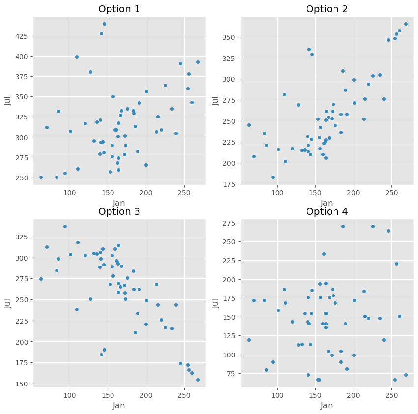
Option 1
Option 2
Option 3
Option 4
Answer: Option 1
Since r = \frac{2}{5}, the correct option must be a scatter plot with a mild positive (up and to the right) linear association. Option 3 can be ruled out immediately, since the linear association in it is negative (down and to the right). Option 2’s linear association is too strong for r = \frac{2}{5}, and Option 4’s linear association is too weak for r = \frac{2}{5}, which leaves Option 1.
The average score on this problem was 57%.
Suppose the standard deviation of the number of sunshine hours in January for cities in California is equal to the standard deviation of the number of sunshine hours in July for cities in California.
Raine’s hometown of Santa Clarita saw 60 more sunshine hours in January than the average California city did. How many more sunshine hours than average does the regression line predict that Santa Clarita will have in July? Give your answer as a positive integer. (Hint: You’ll need to use the fact that the correlation between the two variables is \frac{2}{5}.)
Answer: 24
At a high level, we’ll start with the formula for the regression line in standard units, and re-write it in a form that will allow us to use the information provided to us in the question.
Recall, the regression line in standard units is
\text{predicted }y_{\text{(su)}} = r \cdot x_{\text{(su)}}
Using the definitions of \text{predicted }y_{\text{(su)}} and x_{\text{(su)}} gives us
\frac{\text{predicted } y - \text{mean of }y}{\text{SD of }y} = r \cdot \frac{x - \text{mean of }x}{\text{SD of }x}
Here, the x variable is sunshine hours in January and the y variable is sunshine hours in July. Given that the standard deviation of January and July sunshine hours are equal, we can simplifies our formula to
\text{predicted } y - \text{mean of }y = r \cdot (x - \text{mean of }x)
Since we’re asked how much more sunshine Santa Clarita will have in July compared to the average, we’re interested in the difference y - \text{mean of} y. We were given that Santa Clarita had 60 more sunshine hours in January than the average, and that the correlation between the two variables(correlation coefficient) is \frac{2}{5}. In terms of the variables above, then, we know:
x - \text{mean of }x = 60.
r = \frac{2}{5}.
Then,
\text{predicted } y - \text{mean of }y = r \cdot (x - \text{mean of }x) = \frac{2}{5} \cdot 60 = 24
Therefore, the regression line predicts that Santa Clarita will have 24 more sunshine hours than the average California city in July.
The average score on this problem was 68%.
As we know, San Diego was particularly cloudy this May. More generally, Anthony, another California native, feels that California is getting cloudier and cloudier overall.
To imagine what the dataset may look like in a few years, Anthony subtracts 5 from the number of sunshine hours in both January and July for all California cities in the dataset – i.e., he subtracts 5 from each x value and 5 from each y value in the dataset. He then creates a regression line to use the new xs to predict the new ys.
What is the slope of Anthony’s new regression line?
Answer: \frac{2}{5}
To determine the slope of Anthony’s new regression line, we need to understand how the modifications he made to the dataset (subtracting 5 hours from each x and y value) affect the slope. In simple linear regression, the slope of the regression line (m in y = mx + b) is calculated using the formula:
m = r \cdot \frac{\text{SD of y}}{\text{SD of x}}
r, the correlation coefficient between the two variables, remains unchanged in Anthony’s modifications. Remember, the correlation coefficient is the mean of the product of the x values and y values when both are measured in standard units; by subtracting the same constant amount from each x value, we aren’t changing what the x values convert to in standard units. If you’re not convinced, convert the following two arrays in Python to standard units; you’ll see that the results are the same.
x1 = np.array([5, 8, 4, 2, 9])
x2 = x1 - 5
Furthermore, Anthony’s modifications also don’t change the standard deviations of the x values or y values, since the xs and ys aren’t any more or less spread out after being shifted “down” by 5. So, since r, \text{SD of }y, and \text{SD of }x are all unchanged, the slope of the new regression line is the same as the slope of the old regression line, pre-modification!
Given the fact that the correlation coefficient is \frac{2}{5} and the standard deviation of sunshine hours in January (\text{SD of }x) is equal to the standard deviation of sunshine hours in July (\text{SD of }y), we have
m = r \cdot \frac{\text{SD of }y}{\text{SD of }x} = \frac{2}{5} \cdot 1 = \frac{2}{5}
The average score on this problem was 73%.
Suppose the intercept of Raine’s original regression line – that is, before Anthony subtracted 5 from each x and each y – was 10. What is the intercept of Anthony’s new regression line?
-7
-5
-3
0
3
5
7
Answer: 7
Let’s denote the original intercept as b and the new intercept in the new dataset as b'. The equation for the original regression line is y = mx + b, where:
When Anthony subtracts 5 from each x and y value, the new regression line becomes y - 5 = m \cdot (x - 5) + b'
Expanding and rearrange this equation, we have
y = mx - 5m + 5 + b'
Remember, x and y here represent the number of sunshine hours in January and July, respectively, before Anthony subtracted 5 from each number of hours. This means that the equation for y above is equivalent to y = mx + b. Comparing, we see that
-5m + 5 + b' = b
Since m = \frac{2}{5} (from the previous part) and b = 10, we have
-5 \cdot \frac{2}{5} + 5 + b' = 10 \implies b' = 10 - 5 + 2 = 7
Therefore, the intercept of Anthony’s new regression line is 7.
The average score on this problem was 34%.
Jasmine is trying to get as far away from Anthony as possible and has a trip to Chicago planned after finals. Chicago is known for being very warm and sunny in the summer but cold, rainy, and snowy in the winter. She decides to build a regression line that uses month of the year (where 1 is January, 2 is February, 12 is December, etc.) to predict the number of sunshine hours in Chicago.
What would you expect to see in a residual plot of Jasmine’s regression line?
A patternless cloud of points
A distinctive pattern in the residual plot
Heteroscedasticity (residuals that are not evenly vertically spread)
Answer: A distinctive pattern in the residual plot
We’re told in the problem that the number of sunshine hours per month in Chicago increases from the winter (January) to the summer (July/August) and then decreases again to the winter (December). Here’s a real plot of this data; we don’t need real data to answer this question, but this is the kind of plot you could sketch out in the exam given the description in the question. (The gold shaded area is irrelevant for our purposes.)
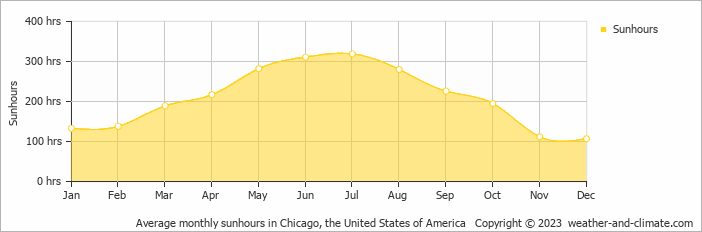
The points in this plot aren’t tightly clustered around a straight line, and that’s because there’s a non-linear relationship between month and number of sunshine hours. As such, when we draw a straight line through this scatter plot, it won’t be able to fully capture the relationship being shown. It’ll likely start off in the bottom left and increase to the top right, which will lead to the sunshine hours for summer months being underestimated and the sunshine hours for later winter months (November, December) being overestimated. This will lead to a distinctive pattern in our residual plot, which means that linear regression as-is isn’t the right tool for modeling this data (because ideally, the residual plot would be a patternless cloud of points).
The average score on this problem was 47%.