← return to practice.dsc10.com
Instructor(s): Janine Tiefenbruck
This exam was administered in-person. The exam was closed-notes, except students were provided a copy of the DSC 10 Reference Sheet. No calculators were allowed. Students had 3 hours to take this exam.
⚠️ PDF version available here .
Note (groupby / pandas 2.0): Pandas 2.0+ no longer
silently drops columns that can’t be aggregated after a
groupby, so code written for older pandas may behave
differently or raise errors. In these practice materials we use
.get() to select the column(s) we want after
.groupby(...).mean() (or other aggregations) so that our
solutions run on current pandas. On real exams you will not be penalized
for omitting .get() when the old behavior would have
produced the same answer.
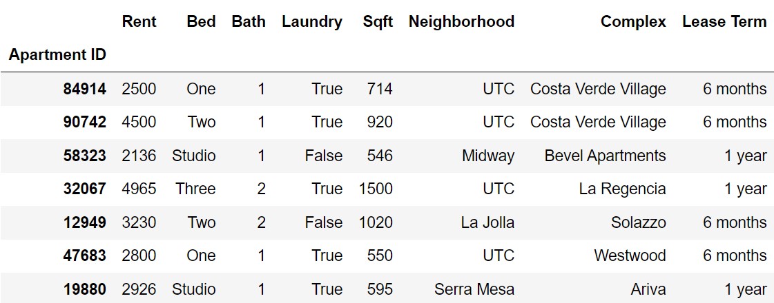
In this final, we’ll explore data on 800 different apartments
available for rent in San Diego. Each row in the DataFrame
apts corresponds to an individual apartment. The DataFrame
is indexed by "Apartment ID" (int), which is a
unique identifier for the apartment.
The columns of apts are as follows:
"Rent" (int): The monthly rent for the
apartment, in dollars."Bed" (str): The number of bedrooms in the
apartment. Values are "Studio", "One",
"Two", and "Three"."Bath" (str): The number of bathrooms in
the apartment. Values are "One",
"One and a half", "Two",
"Two and a half", and "Three"."Laundry" (bool): If the apartment comes
with an in-unit washer and dryer."Sqft" (int): The area of the apartment,
in square feet."Neighborhood" (str): The neighborhood in
which the apartment is located."Complex" (str): The complex the apartment
is a part of."Lease Term" (str): The duration of the
apartment’s lease. Values are "1 month",
"6 months", and "1 year".The first few rows of apts are shown below, though
apts has many more rows than pictures, 800 in total. The
data in apts is only a sample from the much larger
population of all San Diego apartments.
Throughout this exam, assume that we have already run
import babypandas as bpd and
import numpy as np.
Yutian wants to rent a one-bedroom apartment, so she decides to learn
about the housing market by plotting a density histogram of the monthly
rent for all one-bedroom apartments in the apts DataFrame.
In her call to the DataFrame method .plot, she sets the
bins using the parameter
bins = np.arange(0, 10000, 100)
How many bins will this histogram have?
Answer: 99
np.arange(start, stop, step) takes the following three
parameters as arguments.
start: The starting value of the sequence
(inclusive).stop: The last value of the sequence (exclusive).step: The difference between each two consecutive
values.This means that np.arange(0, 10000, 100) will create a
NumPy array that starts at 0, and ends before it reaches 10000 - all
while incrementing by 100 for each step. To calculate the number of bins
within the parameter, we can write \frac{\text{stop} - \text{start}}{\text{step}} -
1.
Another way we can look at this is by taking a small sample of this
sequence (such as np.arange(0, 300, 100)). This will create
the array np.array([0, 100, 200]) without including the
stop argument (300). Note that the same equation holds true.
Note: Mathematically,
np.arange(start, stop) can be represented as [\text{start}, \text{stop})
The average score on this problem was 64%.
Suppose there are 300 one-bedroom apartments in the apts
DataFrame, and 15 of them cost between $2,300 (inclusive) and $2,400
(exclusive). How tall should the bar for the bin [2300, 2400) be in the density histogram?
Give your answer as a simplified fraction or exact decimal.
Answer: 0.0005 = \frac{1}{2000}
Before we start, we need to take note that the question is asking for the density of the bin, since we are representing the data in a density histogram. In order to calculate the density of the bin we use the following equation:
\frac{\text{Number of points in the bin}}{\text{Total number of points} \cdot \text{Width of bin}}
To solve, we plug in the following values into the equation:
\frac{15}{300 \cdot 100} = \frac{1}{20 \cdot 100} = \frac{1}{2000}
Therefore, the density of this bin is \frac{1}{2000}
The average score on this problem was 51%.
Suppose some of the one-bedroom apartments in the apts
DataFrame cost more than $5,000. Next, Yutian plots another density
histogram with
bins = np.arange(0, 5000, 100)
Consider the bin [2300, 2400) in
this new histogram. Is it taller, shorter, or the same height as in the
old histogram, where the bins were
np.arange(0, 10000, 100)?
Taller
Shorter
The same height
Not enough information to answer
Answer: Taller
In this histogram, we will only have data that that fits within the constraints of [0, 5000). Since we are told that there are apartments that fit outside of the constraint, there will be an overall smaller number of points points represented by the histogram.
Taking the histogram density estimation equation, \frac{\text{Number of points in the bin}}{\text{Total number of points} \cdot \text{Width of bin}}, we know that our total number of points have decreased (with respect to the constraints shown in the bins). So, a smaller denominator would lead to a proportional increase in the resulting product. Because the resulting product increases, this means that the height of this particular bin will be taller.
The average score on this problem was 55%.
Michelle and Abel are each touring apartments for where they might
live next year. Michelle wants to be close to UCSD so she can attend
classes easily. Abel is graduating and wants to live close to the beach
so he can surf. Each person makes their own DataFrame (called
michelle and abel respectively), to keep track
of all the apartments that they toured. Both michelle and
abel came from querying apts, so both
DataFrames have the same columns and structure as apts.
Here are some details about the apartments they toured.
We’ll assume for this problem only that there is just one apartment
of each size available at each complex, so that if they both tour a one
bedroom apartment at the same complex, it is the exact same apartment
with the same "Apartment ID".
What does the following expression evaluate to?
michelle.merge(abel, left_index=True, right_index=True).shape[0]Answer: 8
This expression uses the indices of michelle and
abel to merge. Since both use the index of
"Apartment ID" and we are assuming that there is only one
apartment of each size available at each complex, we only need to see
how many unique apartments michelle and abel
share. Since there are 8 complexes that they both visited, only the one
bedroom apartments in these complexes will be displayed in the resulting
merged DataFrame. Therefore, we will only have 8 apartments, or 8
rows.
The average score on this problem was 48%.
What does the following expression evaluate to?
michelle.merge(abel, on=“Bed”).shape[0]
Answer: 240
This expression merges on the "Bed" column, so we need
to look at the data in this column for the two DataFrames. Within this
column, michelle and abel share only one
specific type of value: "One". With the details that are
given, michelle has 12 rows containing this value while
abel has 20 rows containing this value. Since we are
merging on this row, each row in abel that contains the
"One" value will be matched with a row in
michelle that also contains the value, meaning one row in
michelle will turn into twelve after the merge.
Thus, to compute the total number of rows from this merge expression,
we multiply the number of rows in michelle with the number
of rows in abel that fit the cross-criteria of
"Bed". Numerically, this would be 12 \cdot 20 = 240.
The average score on this problem was 33%.
What does the following expression evaluate to?
michelle.merge(abel, on=“Complex”).shape[0] Answer: 32
To approach this question, we first need to determine how many
complexes Michelle and Abel have in common: 8. We also know that each
complex was toured twice by both Michelle and Abel, so there are two
copies of each complex in the michelle and
abel DataFrames. Therefore, when we merge the DataFrames,
the two copies of each complex will match with each other, effectively
creating four copies for each complex from the original two. Since this
is done for each complex, we have 8 \cdot (2
\cdot 2) = 32.
The average score on this problem was 19%.
What does the following expression evaluate to?
abel.merge(abel, on=“Bed”).shape[0]
Answer: 800
Since this question deals purely with the abel
DataFrame, we need to fully understand what is inside it. There are 40
apartments (or rows): 20 one bedrooms and 20 two bedrooms. When we
self-merge on the "Bed" column, it is imperative to know
that every one bedroom apartment will be matched with the 20 other one
bedroom apartments (including itself)! This also goes for the two
bedroom apartments. Therefore, we have 20
\cdot 20 + 20 \cdot 20 = 800.
The average score on this problem was 28%.
We wish to compare the average rent for studio apartments in different complexes.
Our goal is to create a DataFrame studio_avg where each
complex with studio apartments appears once. The DataFrame should
include a column named "Rent" that contains the average
rent for all studio apartments in that complex. For each of the
following strategies, determine if the code provided works as intended,
gives an incorrect answer, or errors.
studio = apts[apts.get("Bed") == "Studio"]
studio_avg = studio.groupby("Complex").mean().reset_index()
Works as intended
Gives an incorrect answer
Errors
studio_avg = apts.groupby("Complex").min().reset_index()Works as intended
Gives an incorrect answer
Errors
grouped = apts.groupby(["Bed", "Complex"]).mean().reset_index()
studio_avg = grouped[grouped.get("Bed") == "Studio"]
Works as intended
Gives an incorrect answer
Errors
grouped = apts.groupby("Complex").mean().reset_index()
studio_avg = grouped[grouped.get("Bed") == "Studio"]
Works as intended
Gives an incorrect answer
Errors
Answer:
studio is set to a DataFrame that is queried from the
apts DataFrame so that it contains only rows that have the
"Studio" value in "Bed". Then, with
studio, it groups by the "Complex" and
aggregates by the mean. Finally, it resets its index. Since we have a
DataFrame that only has "Studio"s , grouping by the
"Complex" will take the mean of every numerical column -
including the rent - in the DataFrame per "Complex",
effectively reaching our goal.
The average score on this problem was 96%.
studio_avg is created by grouping
"Complex" and aggregating by the minimum. However, as the
question asks for the average rent, getting the minimum
rent of every complex does not reach the conclusion the question asks
for.
The average score on this problem was 95%.
grouped is made through first grouping by both the
"Bed" and "Complex" columns then taking the
mean and resetting the index. Since we are grouping by both of these
columns, we separate each type of "Bed" by the
"Complex" it belongs to while aggregating by the mean for
every numerical column. After resetting the index, we are left with a
DataFrame that contains the mean of every "Bed" and
"Complex" combination. A sample of the DataFrame might look
like this:| Bed | Complex | Rent | … |
|---|---|---|---|
| One | Costa Verde Village | 3200 | … |
| One | Westwood | 3000 | … |
| … | … | … | … |
Then, when we assign studio_avg, we take this DataFrame
and only get the rows in which grouped’s "Bed"
column contains "Studio". As we already
.groupby()’d and aggregated by the mean for each
"Bed" and "Complex" pair, we arrive at the
solution the question requests for.
The average score on this problem was 84%.
grouped, we only .groupby() the
"Complex" column, aggregate by the mean, and reset index.
Then, we attempt to assign studio_avg to the resulting
DataFrame of a query from our grouped DataFrame. However,
this wouldn’t work at all because when we grouped by
"Complex" and aggregated by the mean to create
grouped, the .groupby() removed our
"Bed" column since it isn’t numerical. Therefore, when we
attempt to query by "Bed", babypandas cannot locate such
column since it was removed - resulting in an error.
The average score on this problem was 60%.
Consider the DataFrame alternate_approach defined as
follows
grouped = apts.groupby(["Bed", "Complex"]).mean().reset_index()
alternate_approach = grouped.groupby("Complex").min()
Suppose that the "Rent" column of
alternate_approach has all the same values as the
"Rent" column of studio_avg, where
studio_avg is the DataFrame described in part (a). Which of
the following are valid conclusions about apts? Select all
that apply.
No complexes have studio apartments.
Every complex has at least one studio apartment.
Every complex has exactly one studio apartment.
Some complexes have only studio apartments.
In every complex, the average price of a studio apartment is less than or equal to the average price of a one bedroom apartment.
In every complex, the single cheapest apartment is a studio apartment.
None of these.
Answer: Options 2 and 5
alternate approach first groups by "Bed"
and "Complex" , takes the mean of all the columns, and
resets the index such that "Bed" and "Complex"
are no longer indexes. Now there is one row per "Bed" and
"Complex" combination that exists in apts and
all columns contain the mean value for each of these "Bed"
and "Complex" combinations. Then it groups by
"Complex" again, taking the minimum value of all columns.
The output is a DataFrame indexed by "Complex" where the
"Rent"column contains the minimum rent (from of all the
average prices for each type of "Bed").
"Rent" column in alternate_approachin contains
the minimum of all the average prices for each type of
"Bed" and the "Rent" column in
"studio_avg" contains the average rent for studios in each
type of complex. Even though they contain the same values, this does not
mean that no studios exist in any complexes. If this were the case,
studio_avg would be an empty DataFrame and
alternate_approach would not be.alternate_approach would not
appear in studio_avg.studio_avg has the average of
all these studios for each complex and alternate_approach
will have the minimum rent (from all the average prices for each type of
bedroom). Just because the columns are the same does not mean that there
is only one studio per complex.studio_avg contains the average
price for a studio in each complex. alternate_approach
contains the minimum rent from the average rents of all types of
bedrooms for each complex. Since these columns are the same, this means
that the average price of a studio must be lower (or equal to) the
average price of a one bedroom (or any other type of bedroom) for all
the rent values in alternate_approach to align with all the
values in studio_avg.
The average score on this problem was 73%.
Which data visualization should we use to compare the average prices of studio apartments across complexes?
Scatter plot
Line chart
Bar chart
Histogram
Answer: Bar chart
Each complex is a categorical data type, so we should use a bar chart to compare average prices.
The average score on this problem was 85%.
According to Chebyshev’s inequality, at least 80% of San Diego apartments have a monthly parking fee that falls between $30 and $70.
What is the average monthly parking fee?
Answer: \$50
We are given that the left and right bounds of Chebyshev’s inequality are $30 and $70 respectively. Thus, to find the middle of the two, we compute the following equation (the midpoint equation):
\frac{\text{right} + \text{left}}{2}
\frac{70 + 30}{2} = 50
Therefore, 50 is the average monthly parking fee.
The average score on this problem was 92%.
What is the standard deviation of monthly parking fees?
\frac{20}{\sqrt{5}}
\frac{40}{\sqrt{5}}
20\sqrt{5}
20\sqrt{5}
Answer: \frac{20}{\sqrt{5}}
Chebyshev’s inequality states that at least 1 - \frac{1}{z^2} of values are within z standard deviations of the mean. In addition, z can be represented as \frac{\text{bound} - \text{mean of x}}{\text{SD of x}}.
Therefore, we can set up the equation like so: \frac{4}{5} = 1 - \frac{1}{(\frac{\text{bound} - \text{mean of x}}{\text{SD of x}})^2}
Then, we can solve: \frac{1}{5} = \frac{1}{(\frac{\text{bound} - \text{mean of x}}{\text{SD of x}})^2}
Now since we know both bounds, we can plug one of them in. Since the mean was computed in the earlier step, we also plug this in.
\frac{1}{5} = \frac{1}{(\frac{70 - 50}{\text{SD of x}})^2} 5 = (\frac{20}{\text{SD of x}})^2 \sqrt{5} = \frac{20}{\text{SD of x}} \text{SD of x} = \frac{20}{\sqrt{5}}
The average score on this problem was 70%.
You are given the following information about security deposits for a sample of 400 apartments in the Mission Hills neighborhood of San Diego:
Using the fact that scipy.stats.norm.cdf(-0.8) evaluates
to about 0.21, construct a 58% confidence interval for the mean security
deposit of all Mission Hills apartments. Below, give the endpoints of
your confidence interval, both as integers.
Left endpoint: ____(a)____
Right endpoint: ____(b)____
Answer:
scipy.stats.norm.cdf(-0.8) tells us that from the bounds
of (-\inf, -0.8], the normal
distribution has an area of 0.21.
Therefore, if we take it to the other side from [0.8, \inf), it also has an area of 0.21 due to the symmetrical property of the
normal distribution. This means that the interval between [-0.8, 0.8] has an area of 1 - 0.21 - 0.21 = 0.58: the confidence
interval we are aiming to find.
In the question, we are given the standard deviation of security deposits in a sample, meaning we need to find the standard deviation for the population. To find this, we use the following formula and compute:
\frac{\text{SD of sample}}{\sqrt{\text{sample size}}} = \frac{500}{\sqrt{400}} = \frac{500}{20} = 25.
Now that we have the population standard deviation, we can calculate the endpoints of the confidence interval.
Left endpoint: 2300 - \frac{4}{5} \cdot 25 = 2280
Right endpoint: 2300 + \frac{4}{5} \cdot 25 = 2320
The average score on this problem was 29%.
You want to use the data in apts to test both of the
following pairs of hypotheses:
Pair 1:
Pair 2:
In apts, there are 467 apartments that are either one
bedroom or two bedroom apartments. You perform the following simulation
under the assumption of the null hypothesis.
prop_1bf = np.array([])
abs_diff = np.array([])
for i in np.arange(10000):
    prop = np.random.multinomial(467, [0.5, 0.5])[0]/467
    prop_1br = np.append(prop_1br, prop)
    abs_diff = np.append(abs_diff, np.abs(prop-0.5))
You then calculate some percentiles of prop_1br. The
following four expressions all evaluate to True.
np.percentiles(prop_1br, 2.5) == 0.4
np.percentiles(prop_1br, 5) == 0.42
np.percentiles(prop_1br, 95) == 0.58
np.percentiles(prop_1br, 97.5) == 0.6What is prop_1br.mean() to two decimal places?
Answer: 0.5
From the given percentiles, we can notice that since the distribution is symmetric around the mean, the mean should be around the 50th percentile. Given the symmetry and the percentiles around 0.5, we can infer that the mean should be very close to 0.5.
Another way we can look at it is by noticing that prop
is pulled from a [0.5, 0.5]
distribution (because we are simulating under the null hypotheses) in
np.random.multinomial(). This means that its expected for
most of the distribution to be from around 0.5.
The average score on this problem was 84%.
What is np.std(prop_1br) to two decimal places?
Answer: 0.05
If we look again at the percentiles, we notice that it seems to resemble a normal distribution. So by taking the mean and the 97.5th percentile, we can solve for the standard deviation. Since [2.5, 97.5] is the 95% confidence interval, we can say that the 97.5th percentile is two standard deviations away from the mean (2.5 too!). Thus,
0.5 + 2 \cdot \text{SD} = 0.6
\therefore Solving for SD, we get \text{SD} = 0.05
The average score on this problem was 45%.
What is np.percentile(abs_diff, 95) to two decimal
places?
Answer: 0.1
Each time through our for-loop, we execute the following lines of code:
prop_1br = np.append(prop_1br, prop)
abs_diff = np.append(abs_diff, np.abs(prop-0.5))
Additionally, we’re told the following statements evaluate to True:
np.percentiles(prop_1br, 2.5) == 0.4
np.percentiles(prop_1br, 5) == 0.42
np.percentiles(prop_1br, 95) == 0.58
np.percentiles(prop_1br, 97.5) == 0.6
We can combine these pieces of information to find the answer to this question.
First, consider the shape of the distribution of
prop_1br. We know it’s symmetrical around 0.5, and beyond
that, we can infer that it’s a normal distribution.
Now, think about how this relates to the distribution of
abs_diff. abs_diff is generated by finding the
absolute difference between prop_1br and 0.5. Because of
this, abs_diff is an array of distances (which are nonnegative by
definition) from 0.5.
We know that prop_1br is normal, and symmetrical about
0.5. So, the distribution of how far away prop_1br is from
0.5 will look like we took the distribution of prop_1br,
moved it to be centered at 0, and folded it in half so that all negative
values become positive. This is because the previous center at 0.5
represents a distance of 0 from 0.5. Similarly, a value of 0.6 would
represent a distance of 0.1 from 0.5, and a value of 0.4 would also
represent a distance of 0.1 from 0.5.
Now, the problem becomes much simpler to solve. Before, we were told
that 95% of our the in prop_1br lies between 0.4 and 0.6
(Thanks to the lines of code that evaluate to True). This is the same as
telling us that 95% of the data in prop_1br lies within a
distance of 0.1 to 0.5 (Because 0.4 and 0.6 are both 0.1 away from
0.5).
Because of this, the 95% percentile of abs_diff is 0.1, since 95% of
the data in prop_1br lies within a distance of 0.1 to 0.5
(meaning that 95% of the data in abs_diff is between 0 and 0.1).
The average score on this problem was 10%.
Which simulated test statistics should be used to test the first pair of hypotheses?
prop_1br
abs_diff
Answer: prop_1br
Our first pair of hypotheses’ alternative hypothesis asks if one number is greater than the other. Because of this, we can’t use an absolute value test statistic to answer the question, since all absolute value cares about is the distance the simulation is from the null assumption, not whether one value is greater than the other.
The average score on this problem was 82%.
Which simulated test statistics should be used to test the second pair of hypotheses?
prop_1br
abs_diff
Answer: abs_diff
Our first pair of hypotheses’ alternative hypothesis asks if one number is not equal to the other. Because of this, we have to use a test statistic that sees the distance both ways, not just in one direction. Therefore, we use the absolute value.
The average score on this problem was 83%.
Your observed data in apts is such that you reject the
null for the first pair of hypotheses at the 5% significance level, but
fail to reject the null for the second pair at the 5% significance
level. What could the value of the following proportion have been?
\frac{\text{\# of one bedroom apartments in \texttt{apts}}}{\text{\# of one bedroom apartments in \texttt{apts}+ \# of two bedroom apartments in \texttt{apts}}}
Give your answer as a number to two decimal places.
Answer: 0.59
The average score on this problem was 20%.
You want to know how much extra it costs, on average, to have a
washer and dryer in your apartment. Since this cost is built into the
monthly rent, it isn’t clear how much of your rent will be going towards
this convenience. You decide to bootstrap the data in apts
to estimate the average monthly cost of having in-unit laundry.
Fill in the blanks to generate 10,000 bootstrapped estimates for the average montly cost of in-unit laundry.
yes = apts[apts.get("Laundry")]
no = apts[apts.get("Laundry") == False]
laundry_stats = np.array([])
for i in np.arange(10000):
    yes_resample = yes.sample(__(a)__, __(b)__)
    no_resample = no.sample(__(c)__, __(d)__)
    one_stat = __(e)__
laundry_stats = np.append(laundry_stats, one_stat)Answer:
yes.shape[0]replace=Trueno.shape[0]replace=Trueyes_resample.get("Rent").mean() - no_resample.get("Rent").mean()For both yes_resample and no_resample, we
need to use their respective DataFrames to create a bootstrapped
estimate. Therefore, we randomly sample from their respective DataFrames
with replacement (the law of bootstrap). Then, to calculate the test
statistic, we need to look back at what the question asks of us: to
estimate the average monthly cost of having in-unit
laundry, so we subtract the mean of the bootstrapped estimate
for no (no_resample) from the mean of the
bootstrapped estimate for yes
(yes_resample).
The average score on this problem was 79%.
What if you wanted to instead estimate the average yearly cost of having in-unit laundry?
Below, change the blank (e), such that the procedure not generates 10,000 bootstrapped estimates for the average yearly cost of in-unit laundry.
Suppose you ran your original code from part (a) and used the results to calculate a confidence interval for the average monthly cost of in-unit laundry, which came out to be
[L_M, R_M].
Then, you changed blank (e) as you described above, and ran the code again to calculate a different confidence interval for the average yearly cost of in-unit laundry, which came out to be
[L_Y, R_Y].
Which of the following is the best description of the relationship between the endpoints of these confidence intervals? Note that the symbol \approx means “approximately equal.”
L_Y = 12 \cdot L_M and R_Y = 12 \cdot R_M
L_Y \approx 12 \cdot L_M and R_Y \approx 12 \cdot R_M
L_M = 12 \cdot L_Y and R_M = 12 \cdot R_Y
L_M \approx 12 \cdot L_Y and R_M \approx 12 \cdot R_Y
None of these.
Answer:
12 * (yes_resample.get("Rent").mean() - no_resample.get("Rent").mean())For both L_Y and R_Y, we cannot say that we certainly know that it will be precisely 12 times the value of the average monthly cost. Because every month and year has variablity/noise, we cannot say for certain that it will most definitely be 12 times the value of average monthly cost, but instead will probably be approximately equal.
The bottom two choices flip the inequality and state that the average monthly cost is 12 times the value of the average yearly cost, which would be vastly different from one another.
The average score on this problem was 85%.
The average score on this problem was 79%.
You’re concerned about the validity of your estimates because you think bigger apartments are more likely to have in-unit laundry for one bedroom apartments only.
If your concern is valid and it is true that bigger apartments are
more likely to have in-unit laundry, how will your bootstrapped
estimates for the average monthly cost of in-unit laundry for one
bedroom apartments only compare to the values you computed in part (a)
based on all the apts?
The estimates will be about the same.
The estimates will be generally larger than those you computed in part (a).
The estimates will be generally smaller than those you computed in part (a).
Answer: The estimates will be generally smaller than those you computed in part (a).
If we query the yes and no DataFrames to
contain only one bedroom apartments, the average "Rent" of
these two DataFrames will probably be smaller than the original
DataFrames. Because these two DataFrames now have a smaller mean, their
bootstraps are also likely to also be smaller than what it originally
was.
Another way we can think of it is by first calling our original
yes and no DataFrames as
yes_population and no_population respectively.
Now, if we take yes_population and
no_population on a histogram, we’ll likely see higher
magnitude "Rent" outliers. By removing these outliers, we
are now in a scenario similar to what the question asks. By taking this
smaller subset that doesn’t have outliers and bootstrap, we will most
likely get a smaller estimate than that seen from
yes_population and no_population
bootstraps.
The average score on this problem was 80%.
Consider the distribution of laundry_stats as computed
in part (a). How would this distribution change if we:
The distribution would be wider.
The distribution would be narrower.
The distribution would not change significantly.
apts?The distribution would be wider.
The distribution would be narrower.
The distribution would not change significantly.
Answer:
When the number of repetitions are increased, the overall distribution will end up looking the same. If anything, increasing the number of repetitions would make the bootstrap distribution look more like the true population distribution.
If only half of the rows are used, there would be more variability in the bootstrap, leading to a wider distribution.
The average score on this problem was 36%.
The average score on this problem was 72%.
The management of the Solazzo apartment complex is changing the comple’s name to be the output of the following line of code. Write the new name of this complex as a string.
Note that the string method .capitalize() converts the
first character of a string to uppercase.
("Solazzo".replace("z", "ala" * 2)
          .split("aa")[-1]
          .capitalize()
.replace("o", "Jo"))Answer: “LaJo”
Let’s trace the steps:
We start with the original string: “Solazzo”.
"Solazzo".replace("z", "ala" * 2)
Replace every
instance of “z” with “alaala” since “ala” * 2 = “alaala”:
“Solaalaalaalaalao”
"Solaalaalaalaalao".split("aa")
Split the string by
“aa”: [“Sol”, “l”, “l”, “l”, “lao”]
["Sol", "l", "l", "l", "lao"][-1]
Get the last
element of the list: “lao”
"lao".capitalize()
Uppercase the first character of
the string: “Lao”
"Lao".replace("o", "Jo")
Replace every instance of
“o” with “Jo”: “LaJo”
The average score on this problem was 76%.
The management fo the Renaissance apartment complex has decided to follow suit and rename their complex to be the output of the following line of code. Write the new name of this complex as a string.
(("Renaissance".split("n")[1] + "e") * 2).replace("a", "M")Answer: “MissMeMissMe”
Let’s trace the steps:
We start with the original string: “Renaissance”.
"Renaissance".split("n")
Split the string by “n”:
[“Re”, “aissa”, “ce”]
["Re", "aissa", "ce"][1]
Get the element in the 1st
index of the list (the second element in the list): “aissa”
"aissa" + e
Add an “e” to the end of the string:
“aissae”
("aissae") * 2
Repeat the string twice:
“aissaeaissae”
"aissaeaissae".replace("a", "M")
Replace every
instance of “a” with “M”: “MissMeMissMe”
The average score on this problem was 70%.
For each expression below, determine the data type of the output and the value of the expression, if possible. If there is not enough information to determine the expression’s value, write “Unknown” in the corresponding blank.
apts.get("Rent").iloc[43] * 4 / 2
Answer:
We know that all values in the column Rent are
ints. So, when we call .iloc[43] on this
column (which grabs the 44th entry in the column), we know the result
will be an int. We then perform some multiplication and
division with this value. Importantly, when we divide an
int, the type is automatically changed to a
float, so the type of the final output will be a
float. Since we do not explicitly know what the 44th entry
in the Rent column is, the exact value of this
float is unknown to us.
The average score on this problem was 77%.
apts.get("Neighborhood").iloc[2][-3]
Answer:
This code takes the third entry (the entry at index 2) from the
Neighborhood column of apts, which is a
str, and it takes the third to last letter of that string.
The third entry in the Neighborhood column is
'Midway', and the third to last letter of
'Midway' is 'w'. So, our result is a
string with value w.
The average score on this problem was 73%.
(apts.get("Laundry") + 5).max()
Answer:
This code deals with the Laundry column of
apts, which is a Series of Trues and
Falses. One property of Trues and
Falses is that they are also interpreted by Python as ones
and zeroes. So, the code (apts.get("Laundry") + 5).max()
adds five to each of the ones and zeroes in this column, and then takes
the maximum value from the column, which would be an int of
value 6.
The average score on this problem was 69%.
apts.get("Complex").str.contains("Verde")
Answer:
This code takes the column (series) "Complex" and
returns a new series of True and False values.
Each True in the new column is a result of an entry in the
"Complex" column containing "Verde". Each
False in the new column is a result of an entry in the
"Complex" column failing to contain "Verde".
Since we are not given the entirety of the "Complex"
column, the exact value of the resulting series is unknown to us.
The average score on this problem was 64%.
apts.get("Sqft").median() > 1000
Answer:
This code finds the median of the column (series) "Sqft"
and compares it to a value of 1000, resulting in a bool
value of True or False. Since we do not know
the median of the "Sqft" column, the exact value of the
resulting code is unknown to us.
The average score on this problem was 87%.
We want to use the data in apts to test the following
hypotheses:
While we could answer this question with a permutation test, in this problem we will explore another way to test these hypotheses. Since this is a question of whether two samples come from the same unknown population distribution, we need to construct a “population” to sample from. We will construct our “population” in the same way as we would for a permutation test, except we will draw our sample differently. Instead of shuffling, we will draw our two samples with replacement from the constructed “population”. We will use as our test statistic the difference in means between the two samples (in the order UTC minus elsewhere).
Suppose the data in apts, which has 800 rows, includes
85 apartments in UTC. Fill in the blanks below so that
p_val evaluates to the p-value for this hypothesis test,
which we will test according to the strategy outlined above.
diffs = np.array([])
for i in np.arange(10000):
    utc_sample_mean = __(a)__
    elsewhere_sample_mean = __(b)__
    diffs = np.append(diffs, utc_sample_mean - elsewhere_sample_mean)
observed_utc_mean = __(c)__
observed_elsewhere_mean = __(d)__
observed_diff = observed_utc_mean - observed_elsewhere_mean
p_val = np.count_nonzero(diffs __(e)__ observed_diff) / 10000Answer:
apts.sample(85, replace=True).get("Rent").mean()apts.sample(715, replace=True).get("Rent").mean()apts[apts.get("neighborhood")=="UTC"].get("Rent").mean()apts[apts.get("neighborhood")!="UTC"].get("Rent").mean()>=For blanks (a) and (b), we can gather from context (hypothesis test
description, variable names, and being inside of a for loop) that this
portion of our code needs to repeatedly generate samples of size 85 (the
number of observations in our dataset that are from UTC) and size 715
(the number of observations in our dataset that are not from UTC). We
will then take the means of these samples and assign them to
utc_sample_mean and elsewhere_sample_mean. We
can generate these samples, with replacement, from the rows in our
dataframe, hinting that the correct code for blanks (a) and (b) are:
apts.sample(85, replace=True).get("Rent").mean() and
apts.sample(715, replace=True).get("Rent").mean().
For blanks (c) and (d), this portion of the code needs to take our
original dataframe and gather the observed means for apartments from UTC
and apartments not from UTC. We can achieve this by querying our
dataframe, grabbing the rent column, and taking the mean. This implies
our correct code for blanks (c) and (d) are:
apts[apts.get("neighborhood")=="UTC"].get("Rent").mean()
and
apts[apts.get("neighborhood")!="UTC"].get("Rent").mean().
For blank (e), we need to determine, based off of our null and
alternative hypotheses, how we should compare the differences in found
in our simulations against our observed difference. The alternative
indicates that that values of rent of apartments in UTC are
higher than the rent of other apartments in other
neighborhoods. Since the observed statistic is calculated by
observed_utc_mean - observed_elsewhere_mean, we want to use
>= in (e) since greater values of diff
indicate that observed_utc_mean is greater than
observed_elsewhere_mean which is in the direction of the
alternative hypothesis.
The average score on this problem was 70%.
Now suppose we tested the same hypothesses with a permutation test using the same test statistic. Which of your answers above (part a) would need to change? Select all that apply.
blank (a)
blank (b)
blank (c)
blank (d)
blank (e)
None of these.
Answer: Blanks (a) and (b) would need to change. For
a permutation test, we would shuffle the labels in our apts
dataset and find the utc_sample_mean and
elsewhere_sample_mean of this new shuffled dataset. Note
that this process is done without replacement and that
both of these sample means are calculated from the same shuffle
of our dataset.
As it currently stands, our code for blanks (a) and (b) do not reflect this; the current process is sampling with replacement from two different shuffles of our dataset. So, blanks (a) and (b) must change.
The average score on this problem was 93%.
Now suppose we test the following pair of hypotheses.
Then we can test this pair of hypotheses by constructing a 95% confidence interval for a parameter and checking if some particular number, x, falls in that confidence interval. To do this:
What parameter should we construct a 95% confidence interval for? Your answer should be a phrase or short sentence.
What is the value of x? Your answer should be a number.
Suppose x is in the 95% confidence interval we create. Select all valid conclusions below.
We reject the null hypothesis at the 5% significance level.
We reject the null hypothesis at the 1% significance level.
We fail to reject the null hypothesis at the 5% significance level.
We fail to reject the null hypothesis at the 1% significance level.
Answer:
For (i), we need to construct a confidence interval for a parameter that allows us to make assessments about our null and alternative hypotheses. Since these two hypotheses discuss whether or not there exists a difference, on average, for rents of apartments in UTC versus rents of apartments elsewhere, our parameter should be: the difference in rent for apartments in UTC and apartments elsewhere on average, or vice versa (The average rent of an apartment in UTC minus the average rent of an apartment elsewhere, or vice versa.)
For (ii), x must be 0 because the value zero holds special significance in our confidence interval; the inclusion of zero within our confidence interval suggests that “there is no difference between rent of apartments in UTC and apartments elsewhere, on average”. Whether or not zero is included within our confidence interval tells us whether we should fail to reject or reject the null hypothesis.
For (iii), if x = 0 lies within our 95% confidence interval, it suggests that there is a sizable chance that there is no difference between rent of apartments in UTC and apartments elsewhere, on average, which is a conclusion in favor of our null hypothesis; this means that any options which reject the null hypothesis, such as the 1st and 2st options, are wrong. The 3rd option (correctly) fails to the reject the null hypothesis at the 5% significance level, which is exactly what a 95% confidence interval that includes x = 0 would support. The 4th option is also correct because any evidence weak enough to fail to reject the null hypothesis at the 5% significance level will also fail at a tighter, more rigorous significance level (such as 1%).
The average score on this problem was 36%.
The average score on this problem was 53%.
The average score on this problem was 77%.
Next year, six of the DSC tutors (Kathleen, Sophia, Kate, Ashley, Claire, and Vivian) want to rent a 3-bedroom apartment together. Each person will have a single roommate with whom they’ll share a bedroom. They determine the bedroom assignments randomly such that each possible arrangement is equally likely.
For both questions below, give your answer as a simplified fraction or exact decimal.
Hint: Both answers can be expressed in the form \frac{1}{k} for an integer value of k.
What is the probability that Kathleen and Sophia are roommates?
Hint: Think about the problem from the perspective of Kathleen.
Answer: \displaystyle\frac{1}{5}
From Kathleen’s perspective, there are 5 tutors that are equally likely to become her roommate. So, the probability that Sophia ends up being Kathleen’s roommate is \displaystyle\frac{1}{5}.
The average score on this problem was 90%.
What is the probability that the bedroom assignments are the following: Kathleen with Sophia, Kate with Ashley, and Claire with Vivian?
Answer: \frac{1}{15}
In order to get this combination of roommates, we can use similar logic as before. From Kathleen’s perspective, there are 5 tutors that are equally likely to become her roommate. So, the probability that Sophia ends up being Kathleen’s roommate is \displaystyle\frac{1}{5}. From there, we can view the situation from Kate’s perspective; Kate sees that there are 3 potential roommates left (Ashley, Claire, Vivian). So, the probability that Ashley ends up being Kate’s roommate (given Kathleen and Sophia are together) is \displaystyle\frac{1}{3}. After Kate chooses her roommate, Claire and Vivian end up together by process of elimination. We can multiply these two probabilities to receive: \displaystyle\frac{1}{5} \cdot \displaystyle\frac{1}{3} = \displaystyle\frac{1}{15}.
The average score on this problem was 47%.
Suppose you know the following information.
apts is
$3,000 with a standard deviation of $400.apts is 2,000
square feet, with a standard deviation of 100 square feet.For all parts of this quesiton, give your answer as an integer.
Suppose the rents are normally distributed. What is the rent below which 84% of apartments are priced?
Answer: $3,400
We can use the 68-95-99.7 rule to approximate this answer. The 68-95-99.7 rule is a handy shortcut for approximating how much data from a distribution lies below/above/within certain value ranges. It states that, for a normal distribution:
The bottom 84% percent of our apts data is roughly
equivalent to “all data that lies below 1 standard deviation above the
mean.” In this case, let the mean of our distribution be $3,000, and let
the standard deviation be $400; the rent for which 84% of our apartments
are priced is therefore $3,400.
The average score on this problem was 31%.
Sophie’s apartment rents for $5,000. What is this rent in standard units?
Answer: 5
Standard units (or Z-score) is the number of standard deviations an observation is away from the mean of a distribution. In this case, we want to find how many standard deviations ($400) that our observation ($5000) is away from the mean ($3000). The math works out to five standard deviations:
\frac{5000 - 3000}{400} = 5
The average score on this problem was 93%.
Based on what you know about the rent of Sophie’s apartment, use the regression line to predict the square footage of Sophie’s apartment.
Answer: 2450
The correlation coefficient of 0.9 tells us about the slope of the regression line to predict square footage from rent; this means that “for every standard unit traveled right in the x-direction (rent), the regression line heads 0.9 standard units up in the y-direction (square footage).”
Sophie’s apartment rent is $5000 (or five standard units in the x-direction, rent). So, to get our regresion line prediction for the square footage of Sophie’s apartment, we should head 5 \cdot 0.9 = 4.5 standard units upwards from the mean in the y-direction, square footage. The standard deviation for square footage is $100; this implies that the prediction for Sophie’s apartment square footage should be 100 \cdot 4.5 = 450 square feet above the mean (2000 square feet), totaling to a final prediction of 2450 square feet.
The average score on this problem was 66%.
Sophie’s apartment is actually 2,300 square feet. What is the residual of your prediction?
Answer: -150
A residual just measures the difference between the observed and the predicted value. If our observation is 2300 square feet, and our prediction is 2450 square feet, our residual is then -150 square feet.
The average score on this problem was 59%.
Cici’s apartment is 1,800 square feet. Based on this information, use the regression line to predict the rent of Cici’s apartment.
Answer: $2,280
The correlation coefficient of 0.9 also tells us about the slope of the regression line to predict rent from square footage; this means that “for every standard unit traveled right in the x-direction (square footage), the regression line heads 0.9 standard units up in the y-direction (rent).”
Cici’s apartment square footage is 1,800 square feet (or negative two standard units in the x-direction, square footage). So, to get our regresion line prediction for the rent of Cici’s apartment, we should head -2 \cdot 0.9 = -1.8 standard units from the mean in the y-direction, rent. The standard deviation for rent is $400; this implies that the prediction for Cici’s apartment rent should be 400 \cdot -1.8 = 720 square feet below the mean (3000 dollars), totaling to a final prediction of $2280.
The average score on this problem was 23%.
Values in the "Bath" column are "One",
"One and a half", "Two",
"Two and a half", and "Three". Fill in the
blank in the function float_bath that will convert any
string from the "Bath" column into its corresponding number
of bathrooms, as a float. For example,
float_bath("One and a half") should return
1.5.
def float_bath(s):
    if "One" in s:
        n_baths = 1
    elif "Two" in s:
        n_baths = 2
    else:
        n_baths = 3
    if "and a half" in s:
        __(a)__
    return n_baths
What goes in blank (a)?
Answer: n_baths = n_baths + 0.5
The behavior that we want this line of code to have is to work
regardless if the bath string contains "One",
"Two", or "Three". This means we need to have
some way of taking the value that n_baths is already
assigned and adding 0.5 to it. So, our code should read
n_baths = n_baths + 0.5.
The average score on this problem was 92%.
Values in the "Lease Term" column are
"1 month", "6 months", and
"1 year". Fill in the blanks in the function
int_lease() that will convert any string from the
"Lease Term" column to the corresponding length of the
lease, in months, as an integer.
def int_lease(s):
    if s[-1] == "r":
        return __(b)__
    else:
        return __(c)__
What goes in blanks (b) and (c)?
Answer:
(b): 12(c): int(s[0])The code in blank (b) will only be run if the last letter of
s is "r", which only happens when
s = "1 year". So, blank (b) should return
12.
The code in blank (c) will run when s has any value
other than "1 year". This includes only two options:
1 month, and 6 months. In order to get the
corresponding number of the months for these two string values, we just
need to take the first character of the string and convert it from a
str type to an int type. So, blank (c) should
return int(s[0]).
The average score on this problem was 84%.
The average score on this problem was 67%.
Values in the "Bed" column are "Studio",
"One", "Two", and "Three". The
function int_bed provided below converts any string from
the "Bed" column to the corresponding number of bedrooms,
as an integer. Note that "Studio" apartments count as
having 0 bedrooms.
def int_bed(s):
    if s == "Studio":
        return 0
    elif s == "One":
        return 1
    elif s == "Two":
        return 2
    return 3
Using the provided int_bed function, write one line of
code that modifies the "Bed" column of the
apts DataFrame so that it contains integers instead of
strings.
Important: We will assume throughout the rest of
this exam that we have converted the "Bed" column of
apts so that it now contains ints.
Answer:
apts = apts.assign(Bed = apts.get("Bed").apply(int_bed))
The code above takes the “Bed” column, apts.get("Bed"),
and uses .apply(int_bed), which runs each entry through the
int_bed function that we have defined above. All that is
left is to save the result back to the dataframe; this can be done with
.assign().
The average score on this problem was 68%.
Consider the following four slopes.
"Rent" from
"Sqft"."Sqft" from
"Rent"."Rent" from
"Bed""Bed" from
"Rent".Note that we don’t have enough information to calculate all of these slopes, but you should be able to answer the questions below based not on calculations, but on the interpretation of what these slopes represent in the context of housing.
Which of the above slopes do you expect to be the largest?
1
2
3
4
Answer: Option 3.
The largest slope out of these four options will be the slope that represents the greatest increase in y-units per x-unit: m = \dfrac{\Delta y}{\Delta x}.
Option 1, which predicts "Rent" from
"Sqft", has large values for its y-variable
("Rent"), but also has large values for its x-variable
("Sqft"). The resulting slope is not that big, as it is a
fraction of large values over large values.
Option 2, which predicts "Sqft" from
"Rent", is also not that big of a slope for the same
reasons as Option 1 (slope is a fraction of large values over large
values).
Option 3, which predicts "Rent" from "Bed",
has large values for its y-variable ("Rent"), but has small
values for its x-variable ("Bed"). The resulting slope is
incredibly big, as it is a fraction of large values over small
values.
Option 4, which predicts "Bed" from "Rent",
has small values for its y-variable ("Bed"), but has large
values for its x-variable ("Rent"). The resulting slope is
incredibly small, as it is a fraction of small values over large
values.
Of all four options, Option 3 is the largest slope.
The average score on this problem was 71%.
Which of the above slopes do you expect to be the smallest?
Answer: Option 4.
As explained above, Option 4 is the smallest slope.
The average score on this problem was 76%.
Imagine a DataFrame constructed from apts called
bedrooms, which has one row for each bedroom in an
apartment in apts. More specifically, a one bedroom
apartment in apts will appear as one row in
bedrooms, a two bedroom apartment in apts will
appear as two rows in bedrooms, and a three bedroom
apartment in apts will appear as three rows in
bedrooms. Studio apartments will not appear in
bedrooms at all.
The "Apartment ID" column of bedrooms
contains the "Apartment ID" of the apartment in
apts. Notice that this is not the index of
bedrooms since these values are no longer unique. The
"Cost" column of bedrooms contains the rent of
the apartment divided by the number of bedrooms. All rows of
bedrooms with a shared "Apartment ID" should
therefore have the same value in the "Cost" column.
Recall that apts has 800 rows. How many rows does
bedrooms have?
800
More than 800.
Less than 800.
Not enough information.
Answer: Not enough information.
It is entirely possible that bedrooms has more or less
than 800 rows; we don’t have enough info to tell.
If most of the 800 rows in apts are studio apartments,
most rows in apts will not have corresponding rows in
bedrooms (studio apartments are not reflected in
bedrooms). This would lower the total number of rows in
bedrooms to less than 800.
If most of the 800 rows in apts are three-bedroom
apartments, most rows in apts will each have three
corresponding rows in bedrooms. This would increase the
total number of rows in bedrooms to more than 800.
The average score on this problem was 68%.
Suppose no_studio is defined as follows. (Remember, we
previously converted the "Beds" column to integers.)
no_studio = apts[apts.get("Bed") != 0]Which of the following statements evaluate to the same value as the expression below?
bedrooms.get("Cost").mean()Select all that apply.
no_studio.get("Rent").mean()
no_studio.get("Rent").sum() / apts.get("Bed").sum()
(no_studio.get("Rent") / no_studio.get("Bed")).mean()
(no_studio.get("Rent") / no_studio.get("Bed").sum()).sum()
no_studio.get("Rent").mean() / no_studio.get("Bed").mean()
None of these.
Answer: Options 2, 4, and 5.
Let’s refer to bedrooms.get("Cost").mean() as “the
bedroom code” for this solution.
Option 1 is incorrect. Option 1 takes the mean of all non-studio
apartment rents in apts. This value is significantly larger
than what is produced by the bedroom code (average value of the “Cost”
column in bedrooms), since all “Cost” values in
bedrooms are less than or equal to their corresponding
“Rent” values in apts. So, these two expressions cannot be
equal.
Option 2 is correct. We can view the bedroom code as the same as
summing all of the values in the “Cost” column of bedrooms
and dividing by the total number of rows of bedrooms. This
is a fraction; we can make some clever substitutions in this fraction to
show it is the same as the code for Option 2:
\dfrac{\text{sum of ``Cost" in bedrooms}}{\# \text{ of rows in bedrooms}} \to \dfrac{\text{sum of ``Rent" in no}\_\text{studio}}{\# \text{ of rows in bedrooms}} \to \dfrac{\text{sum of ``Rent" in no}\_\text{studio}}{\text{sum of ``Bed" in apts}}
Option 3 is incorrect. The first part of Option 3,
no_studio.get("Rent") / no_studio.get("Bed"), produces a
Series that contains all the values in the “Cost” column of
no_studio, except without duplicated rows for multi-bed
apartments. Taking the .mean() of this look-alike Series is
not the same as taking the .mean() of the bedroom code, so
these two expressions cannot be equal.
Option 4 is correct. We can show the bedroom code is equivalent to the code in Option 4 as follows:
\dfrac{\text{sum of ``Cost" in bedrooms}}{\# \text{ of rows in bedrooms}} \to \dots \to \dfrac{\text{sum of ``Rent" in no}\_\text{studio}}{\text{sum of ``Bed" in apts}} \to
\dfrac{\text{sum of ``Rent" in no}\_\text{studio}}{\text{sum of ``Bed" in no}\_\text{studio}} \to \text{sum} \left( \dfrac{\text{each entry in ``Rent" in no}\_\text{studio}}{\text{sum of ``Bed" in no}\_\text{studio}} \right)
Option 5 is correct. We can show the bedroom code is equivalent to the code in Option 5 as follows:
\dfrac{\text{sum of ``Cost" in bedrooms}}{\# \text{ of rows in bedrooms}} \to \dots \to \dfrac{\text{sum of ``Rent" in no}\_\text{studio}}{\text{sum of ``Bed" in no}\_\text{studio}} \to
\dfrac{\left(\dfrac{\text{sum of ``Rent" in no}\_\text{studio}}{\# \text{ of rows in no}\_\text{studio}}\right)}{\left(\dfrac{\text{sum of ``Bed" in no}\_\text{studio}}{\# \text{ of rows in no}\_\text{studio}}\right)} \to \dfrac{\text{mean of ``Rent" in no}\_\text{studio}}{\text{mean of ``Bed" in no}\_\text{studio}}
The average score on this problem was 53%.
The table below shows the proportion of apartments of each type in each of three neighborhoods. Note that each column sums to 1.
| Type | North Park | Chula Vista | La Jolla |
|---|---|---|---|
| Studio | 0.30 | 0.15 | 0.40 |
| One bedroom | 0.40 | 0.35 | 0.30 |
| Two bedroom | 0.20 | 0.25 | 0.15 |
| Three bedroom | 0.10 | 0.25 | 0.15 |
Find the total variation distance (TVD) between North Park and Chula Vista. Give your answer as an exact decimal.
Answer: 0.2
To find the TVD, we take the absolute differences between North Park and Chula Vista for all rows, sum them, then cut the result in half.
\dfrac{|0.3 - 0.15| + |0.4 - 0.35| + |0.2 - 0.25| + |0.1 - 0.25|}{2} = \dfrac{0.15 + 0.05 + 0.05 + 0.15}{2} = \dfrac{0.4}{2} = 0.2
The average score on this problem was 72%.
Which pair of neighborhoods is most similar in terms of types of housing, as measured by TVD?
North Park and Chula Vista
North Park and La Jolla
Chula Vista and La Jolla
Answer: North Park and La Jolla
The TVD between North Park and La Jolla is the lowest between all pairs of two of these three neighborhoods:
| Pair | TVD |
|---|---|
| North Park and Chula Vista | 0.2 |
| North Park and La Jolla | 0.15 |
| Chula Vista and La Jolla | 0.25 |
This implies that the distributions of apartment types for North Park and La Jolla are the most similar.
The average score on this problem was 94%.
25% of apartments in Little Italy are one bedroom apartments. Based on this information, what is the minimum and maximum possible TVD between North Park and Little Italy? Give your answers as exact decimals.
Answer:
The minimum TVD is 0.15 because:
The maximum TVD is 0.65 because:
The average score on this problem was 49%.
The average score on this problem was 33%.