← return to practice.dsc10.com
Instructor(s): Janine Tiefenbruck
This exam was administered in-person. Students were allowed one page of double-sided handwritten notes. No calculators were allowed. Students had 3 hours to take this exam.
⚠️ PDF version available here .
A band is a group of musicians who regularly perform and record music together. Some of the most successful bands in history have sold hundreds of millions of records and sold out stadiums worldwide, becoming a central part of popular culture.
In this exam, we’ll study a dataset of 400 bands,
which we will treat as a simple random sample from the
population of all bands. The DataFrame bands has one row
for every band in our dataset. The columns are:
"band" (str): The name of the band. This
column has no repeated values."origin" (str): The country where the band
was formed."genre" (str): The primary musical genre,
such as "Rock", "Pop", "Metal",
or "Alternative"."formed" (int): The year the band was
formed."active" (bool): True if
currently active, False if disbanded."member_names" (str): The names of the
members in the most recent lineup."albums" (int): Total number of studio
albums released."top_album_sales" (float): Worldwide sales
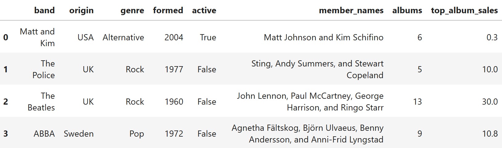
of the band’s best-selling album, in millions of copies.The first few rows of bands are shown below, but
remember that bands has 400 rows.
Throughout this exam, we will refer to bands repeatedly.
Assume that we have already run import babypandas as bpd,
import numpy as np, and import scipy.
[(14 pts)] The column "member_names" is formatted in a
specific way. If a band has two members, the string is of the form
"A and B" with no commas. If the band has three or more
members, names are comma-separated like "A, B, and C" for a
three-person band or "A, B, C, and D" for a four-person
band. Take a look at the first few rows of the DataFrame to make sure
you understand how this column is formatted!
Define the Series names and the function f
as follows.
names = bands.get("member_names")

def f(x):
    return max(x, 2)
Select all expressions below that evaluate to a
Series containing the number of members in each band. Assume that no
band member has a comma (",") in their name, but don’t make
any other assumptions about band members’ names.
names.str.replace(", ", "").str.split(" ").apply(len) - 1
names.str.split(", ").apply(len).apply(f)
(names.str.count(", ") + 1).apply(f)
names.str.replace("and", ", ").str.count(", ").apply(f)
None of the above.
Answer:
Option 2 and Option 3
Solution:
Option 1 is incorrect because splitting on spaces
counts words rather than members. Band members can have multi-word names
such as "John Smith". Subtracting 1 from the word count
does not reliably fix this.
Option 2 is correct because
.str.split(", ") produces one list element per member for
bands with three or more members. A two-member band has no commas, so
its list contains only one element. Applying len counts the
elements, and f takes the maximum of that count and 2,
which corrects the two-member case.
Option 3 is correct because a band with three or
more members has exactly one fewer comma than members, so
.str.count(", ") + 1 gives the right count. A two-member
band has no commas, so the expression gives 1. Applying f
raises this to 2, which is the correct number of members.
Option 4 is incorrect because
.str.replace("and", ", ") replaces every occurrence of
"and", including inside names such as
"Brandon". This inserts extra commas and causes an
overcount. We cannot make assumptions about the names themselves.
Suppose a function g is defined such that
bands.get("member_names").apply(g) evaluates to a Series
containing the number of members in each band. What are the data types
of the input and output to g?
input data type: output data type:
Answer:
strintSolution:
The function g is applied to the Series
bands.get("member_names"), whose values are strings of band
member names, so each input to g is a
string, or str. The purpose of
g is to count the members in each band, and a count is a
whole number, so the output of g is an
integer, or int. Recall that
.apply(g) calls g separately on each value in
the Series, and each returned integer becomes the corresponding value in
the resulting Series.
Fill in the return statement of the function
g as described above.
def g(x):
    return __(a)__
(a):
Answer:
max(x.count(",") + 1, 2)An alternative correct answer is
max(len(x.split(",")), 2).
Solution:
For bands with three or more members, names are separated by commas,
so the member count is x.count(",") + 1. Two-member bands
are separated by " and " with no commas, so this expression
would incorrectly return 1 for them. Since every band has at least two
members, we wrap the expression in max(..., 2) to fix this
case.
def g(x):
    return max(x.count(",") + 1, 2)
Alternatively, len(x.split(",")) gives the same count as
x.count(",") + 1, so max(len(x.split(",")), 2)
also works, assuming names do not contain commas.
Note: For the remainder of the exam, assume that we
have added to bands a new column called
"members" containing the number of members in each
band.
[(10 pts)]
Recall that we have added to bands a new column called
"members" containing the number of members in each
band.
Ella is curious if bands with more members tend to make more albums.
Write one line of code to add a new column to bands called
"albums_per_member", containing the ratio of albums to
members for each band.
1in
Answer:
bands = bands.assign(albums_per_member = bands.get("albums") / bands.get("members"))Solution:
bands.get("albums") / bands.get("members") performs
elementwise division, so each band’s album count is divided by its own
member count, such as 12 albums and 4 members giving \frac{12}{4}=3. The
.assign(albums_per_member = ...) method adds these values
as a new column, and because it returns a new DataFrame rather than
modifying bands in place, we assign the result back to
bands.
bands = bands.assign(albums_per_member = bands.get("albums") / bands.get("members"))Find the year in which the band with the highest
"albums_per_member" ratio was formed. Select
all options that correctly evaluate to this year (or any such
year in the case of a tie).
bands.groupby("albums_per_member").min().sort_values(by=index, ascending=True).iloc[-1]
bands.groupby("albums_per_member").min().reset_index().sort_values(by="albums_per_member", ascending=False).get("formed").iloc[0]
bands.groupby("formed").max().sort_values(by="albums_per_member", ascending=False).get("formed").iloc[0]
bands.groupby("formed").max().sort_values(by="albums_per_member", ascending=False).index[0]
bands.sort_values(by="albums_per_member", ascending=True).get("formed").iloc[-1]
bands.sort_values(by="formed", ascending=False).groupby("albums_per_member").max().index[0]
None of the above.
Answer:
Option 2, Option 4, and Option 5
Solution:
Option 1 is incorrect because index is
not in quotation marks, so sort_values(by=index, ...)
raises an error, and .iloc[-1] would return a whole row
rather than a year.
Option 2 is correct because grouping by
"albums_per_member", resetting the index, sorting in
descending order, and taking .get("formed").iloc[0] returns
a formation year for a band with the highest ratio.
Option 3 is incorrect because
groupby("formed") makes the years the index, so
.get("formed") fails since "formed" is no
longer a column.
Option 4 is correct because after
groupby("formed").max() and a descending sort, the year
with the highest ratio comes first, and .index[0] retrieves
it from the index.
Option 5 is correct because an ascending sort puts
the highest ratio in the last row, so
.get("formed").iloc[-1] gives its year.
Option 6 is incorrect because grouping by
"albums_per_member" makes the ratios the index, so
.index[0] returns a ratio rather than a year.
[(10 pts)]
For each goal below, determine the most appropriate plot type.
Show the relationship between each band’s formation year and
"top_album_sales" to see if older bands tend to have higher
sales.
Scatter plot
Line plot
Bar chart
Answer:
Scatter plot
Solution:
A scatter plot is the most appropriate choice
because both the formation year and "top_album_sales" are
numerical variables, and each point represents one band. It lets us
check for an association between the two, such as a downward trend if
earlier bands tend to have higher sales.
A line plot is less appropriate because we are comparing individual bands rather than tracking a single quantity over time, and connecting the points would imply a sequence that doesn’t exist.
A bar chart is less appropriate because bar charts compare numerical values across categories, whereas both variables here are numerical.
Compare the total number of albums released by bands from each country, with countries sorted from most albums to fewest albums.
Scatter plot
Line plot
Bar chart
Answer:
Bar chart
Solution:
A bar chart is the most appropriate choice because
"origin" is a categorical variable, and we want to compare
a numerical summary, the total number of albums, across countries. We
would group the bands by country, sum the albums for each, and draw one
bar per country, ideally sorted from highest to lowest so the top
countries are easy to spot.
A scatter plot is not appropriate because it displays relationships between two numerical variables, whereas country is categorical.
A line plot is not appropriate because countries have no natural order, and connecting them with lines would suggest a trend that doesn’t exist.
Display how the average number of members in a band has changed over time.
Scatter plot
Line plot
Bar chart
Answer:
Line plot
Solution:
A line plot is the most appropriate choice because we want to see how a numerical quantity changes over time. We would group bands by formation year, compute the average number of members for each year, and plot formation year on the x-axis against that average on the y-axis, with the connecting line making trends in band size easy to spot.
A scatter plot would be better for examining the relationship between formation year and member count across individual bands, rather than a yearly summary.
A bar chart could display the yearly averages, but it is less effective at emphasizing the overall trend across a sequence of years.
Compare "top_album_sales" across different genres to
identify which genre has the highest median sales.
Scatter plot
Line plot
Bar chart
Answer:
Bar chart
Solution:
A bar chart is the most appropriate choice because
genre is a categorical variable, and we want to compare the median
"top_album_sales" across genres. We would group the bands
by genre, compute the median top album sales for each, and draw one bar
per genre, which lets us directly identify the genre with the highest
median.
A scatter plot is less appropriate because it displays relationships between numerical variables, whereas genre is categorical.
A line plot is less appropriate because genres have no natural order, and connecting the medians with lines would suggest a trend that doesn’t exist.
Show the relationship between number of albums released and
"top_album_sales" to see if one variable can be predicted
from the other.
Scatter plot
Line plot
Bar chart
Answer:
Scatter plot
Solution:
A scatter plot is the most appropriate choice
because both the number of albums released and
"top_album_sales" are numerical variables, and each point
represents one band. It lets us examine the direction, strength, and
shape of the association, such as whether bands with more albums tend to
have higher top sales and whether the relationship looks approximately
linear, which is useful for deciding if linear
regression is appropriate.
A line plot is less appropriate because the bands are separate observations rather than a continuous sequence, so connecting them would be misleading.
A bar chart is less appropriate because it compares values across categories rather than investigating the relationship between two numerical variables.
[(8 pts)]
Austin is analyzing the "top_album_sales" column of the
bands DataFrame, which records each band’s best-selling
album sales in millions.
Fill in the blanks so that [lower, upper] is the
interval that contains all values of "top_album_sales" that
fall within 2 standard deviations of the mean.
sales = bands.get("top_album_sales")
lower = __(a)__
upper = __(b)__
(a):
(b):
Answer:
sales.mean() - 2 * np.std(sales)sales.mean() + 2 * np.std(sales)Solution:
An interval containing all values within 2 standard deviations of the
mean extends from 2 standard deviations below the mean
to 2 standard deviations above the mean. We calculate
the mean using sales.mean() and the standard deviation
using np.std(sales). Therefore, the lower bound is
sales.mean() - 2 * np.std(sales), and the upper bound is
sales.mean() + 2 * np.std(sales).
What proportion of "top_album_sales" fall in the
interval [lower, upper]? Choose the best answer below.
Approximately 0.68.
Approximately 0.95.
At least 0.75, but we don’t know exactly.
At least 0.88, but we don’t know exactly.
We cannot determine anything about this proportion.
Answer:
Option 3: At least 0.75, but we don’t know exactly.
Solution:
By Chebyshev’s inequality, for any distribution with
a finite standard deviation, the proportion of values within (k)
standard deviations of the mean is at least (1-). Setting (k=2), we
obtain (1-=0.75), meaning that at least 75% of the values fall within
the interval. Options 1 and 2 refer to the empirical rule for
approximately normal distributions, but we are not told that
"top_album_sales" is normally distributed. Option 4 is
incorrect because Chebyshev’s inequality only guarantees 75% for (k=2),
while Option 5 is incorrect because we can determine this minimum
proportion.
[(17 pts)]
Bianca standardizes the "albums" column, which has a
mean of 7 and a standard deviation of 2 before standardization.
What are the mean and standard deviation of the "albums"
column after standardization?
mean: SD:
Answer:
Solution:
Standardization converts each value into standard units by subtracting the mean and dividing by the standard deviation. This transformation produces a distribution with a mean of 0 and a standard deviation of 1, regardless of the original mean and standard deviation (as long as the original SD is nonzero).
The band Joy Division has an "albums" value
that is -2.5 standard units. How many
albums did this band release?
Answer:
2 albums
Solution:
To convert a standardized value back into its original units, use x = \text{mean} + z \cdot \text{SD}. Substituting the given values, we get x = 7 + (-2.5)(2) = 2. Therefore, Joy Division released 2 albums.
What proportion of bands have an "albums" value in the
interval [5, 9]? Choose the best answer below.
Approximately 0.68.
Approximately 0.95.
At least 0.75, but we don’t know exactly.
At least 0.88, but we don’t know exactly.
We cannot determine anything about this proportion.
Answer:
Option 5: We cannot determine anything about this proportion.
Solution:
The interval [5, 9] extends from one standard deviation
below the mean to one standard deviation above it, since the mean is 7
and the standard deviation is 2. Chebyshev’s inequality
guarantees a proportion of at least 1-\frac{1}{k^2} within k standard deviations, but for k=1, this lower bound is 0 and provides no
useful information. Although approximately 68% of values fall within one
standard deviation of the mean in a normal distribution, we are not told
that the "albums" distribution is normal. Therefore, we
cannot determine the proportion from the information given.
Which of the following could not be the value of a
band’s "albums" in standard units? Select
all that apply.
-4
-0.5
0
1.75
8.5
None of the above.
Answer:
Option 1 and Option 4
Solution:
To convert a value in standard units back to the original number of albums, we use x = 7 + 2z, where z is the standardized value. For Option 1, z=-4 gives x=7+2(-4)=-1, which is impossible because a band cannot release a negative number of albums. For Option 4, z=1.75 gives x=7+2(1.75)=10.5, which is impossible because the number of albums must be a whole number. The remaining values correspond to possible nonnegative integer album counts: -0.5 \rightarrow 6, 0 \rightarrow 7, and 8.5 \rightarrow 24. Therefore, only Options 1 and 4 could not be valid standardized album counts.
[(8 pts)]
Histograms A, B, and C all display the distribution of
"top_album_sales" for the 400 bands in bands,
but they use different bins.
Histogram A uses bins = [0, 10, 20, 30, 40, 50], with
bar heights as follows:
| Bin | Height |
|---|---|
| [0, 10) | 0.03 |
| [10, 20) | 0.02 |
| [20, 30) | 0.01 |
| [30, 40) | 0.03 |
| [40, 50] | 0.01 |
Histogram B uses bins = [0, 20, 40, 50]. Note that not
all bins have the same width. What is the height of the
tallest bar in Histogram B? Give your answer as an
exact decimal.
Answer:
0.025
Solution:
To find each bar’s height in a density histogram, we use \text{Height} = \frac{\text{Proportion}}{\text{Bin Width}}, where the proportion is the area of the bar. Since Histogram B combines bins from Histogram A, we can add the areas of the corresponding bars to calculate each new proportion.
| Bin | Proportion | Width | Height |
|---|---|---|---|
| [0, 20) | 0.50 | 20 | 0.025 |
| [20, 40) | 0.40 | 20 | 0.020 |
| [40, 50] | 0.10 | 10 | 0.010 |
The tallest bar is [0, 20), with a height of 0.025.
Histogram C uses bins = [0, 5, 10, 50], again of varying
widths. Let h_1 be the height of the
leftmost bar, [0, 5). What are the
minimum and maximum possible values of h_1? Give your answers as exact
decimals.
minimum h_1: maximum h_1:
Answer:
Solution:
In Histogram A, the [0, 10) bin has a height of 0.03 and a width of 10, so its area (proportion) is 0.03 \times 10 = 0.30. When this bin is divided into [0, 5) and [5, 10), we do not know how the 0.30 proportion is distributed between the two smaller bins. The minimum possible height occurs when none of the data falls in [0, 5), giving h_1 = \frac{0}{5} = 0. The maximum possible height occurs when all 0.30 of the proportion falls in [0, 5), giving h_1 = \frac{0.30}{5} = 0.06.
[(18 pts)]
Zeyu is wondering whether active bands are more successful than
inactive bands, in the sense that they have greater
"top_album_sales". To find out, he runs a permutation test
on the bands DataFrame by comparing the average
"top_album_sales" for active versus inactive bands using
10,000 shuffles of the "active" labels.
Which of the following best describes the null hypothesis for Zeyu’s test?
Active bands have higher top album sales than inactive bands, on average.
Active bands and inactive bands have the same distribution of top album sales.
In the full population of all bands, the average top album sales for active bands is higher than that for inactive bands.
In the sample of data in bands, the average top album
sales for active bands equals the average top album sales for inactive
bands.
Answer:
Option 2
Solution:
The null hypothesis of a permutation test states that the two groups
come from the same underlying distribution, so the
"active" labels are interchangeable under the null. Option
1 describes the alternative hypothesis that active bands have higher
sales, while Option 3 also describes a population-level alternative
rather than the null. Option 4 is incorrect because the null hypothesis
does not require the two groups to have exactly equal sample means;
differences can occur due to random variation even when the null is
true.
Complete the code below to run Zeyu’s permutation test.
active = bands[bands.get("active") == True].get("top_album_sales")
inactive = bands[bands.get("active") == False].get("top_album_sales")
obs_diff = active.mean() - inactive.mean()

sim_diffs = np.array([])

for i in np.arange(10000):
    shuffled_labels = __(a)__
    shuffled = bands.assign(active=shuffled_labels)
    sim_active = shuffled[shuffled.get("active") == True]
    sim_inactive = shuffled[shuffled.get("active") == False]
    sim_diff = (sim_active.get("top_album_sales").mean()
                - sim_inactive.get("top_album_sales").mean())
    sim_diffs = np.append(sim_diffs, sim_diff)

p_value = __(b)__ / 10000
(a):
(b):
Answer:
np.random.permutation(bands.get("active"))np.count_nonzero(sim_diffs >= obs_diff)Solution:
For (a),
np.random.permutation(bands.get("active")) randomly
rearranges the "active" labels while keeping the number of
active and inactive bands unchanged, breaking any association between
activity status and album sales. Each iteration then calculates the
difference in mean sales between the shuffled active and inactive
groups. For (b), since the alternative hypothesis is
that active bands have higher average sales, we count
simulated differences that are greater than or equal to
the observed difference using
np.count_nonzero(sim_diffs >= obs_diff). Dividing by
10,000 gives the proportion of simulated test statistics at least as
extreme as the observed statistic in the direction of the alternative,
which is the p-value.
Suppose Zeyu’s p-value turns out to be 0.03. Which of the following is the correct conclusion of the test at the 0.05 significance level?
We accept the null hypothesis; active and inactive bands have the same distribution of top album sales.
We fail to reject the null hypothesis; we cannot determine whether the groups differ.
We reject the null hypothesis; active bands have significantly higher top album sales.
We reject the null hypothesis; active and inactive bands have different distributions of top album sales but we can’t say which is greater.
Answer:
Option 3
Solution:
Since the p-value of 0.03 is less than the significance level of 0.05, we reject the null hypothesis. Because the alternative hypothesis is one-sided, the test provides statistically significant evidence that active bands have higher average top album sales than inactive bands. Option 1 is incorrect because we do not “accept” the null hypothesis, and Option 2 is incorrect because the p-value is small enough to reject it. Option 4 is incorrect because the direction of the alternative allows us to conclude that active bands have higher average sales, rather than merely concluding that the groups differ.
In Zeyu’s permutation test, suppose we change the code to instead
shuffle the values in the "top_album_sales" column, and
rerun the simulation. How would this affect the resulting null
distribution?
All 10,000 simulated values would be exactly the same as before.
There would be slight variations in the null distribution but the histogram would look nearly identical.
There would be substantial differences in the null distribution if we were to make this change. The histograms would be noticeably different.
Without the full bands DataFrame available, we cannot
predict how this change would affect the null distribution.
Answer:
Option 2
Solution:
Shuffling the "active" labels and shuffling the
"top_album_sales" values are statistically
equivalent ways of breaking the association between group
membership and album sales while preserving the original group sizes and
sales values. Both methods therefore generate the same theoretical null
distribution for the difference in group means. However, because the
10,000 simulations are random, the individual simulated differences will
not necessarily match between runs, so the resulting histograms should
look nearly identical with only slight random variations.
[(16 pts)]
Sofia is doing research on bands in the UK. She writes the code below to estimate the mean number of members in UK bands using a bootstrapped 85% confidence interval. Fill in the blanks to complete the code.
uk = bands[bands.get("origin") == "UK"]
means = np.array([])

for i in np.arange(5000):
    resample = uk.sample(__(a)__, replace=True)
    means = np.append(means, resample.get("members").mean())

ci_low = np.percentile(means, __(b)__)
ci_high = np.percentile(means, __(c)__)
(a):
(b):
(c):
Answer:
uk.shape[0]7.592.5Solution:
Each bootstrap resample must contain the same number of rows as the
original DataFrame uk, so we use uk.shape[0].
For an 85% confidence interval, we want the middle 85% of the bootstrap
means, leaving 15% outside the interval. Splitting this equally between
the two tails gives 7.5% in each tail. Therefore, we use the
7.5th percentile for the lower endpoint and the
92.5th percentile for the upper endpoint.
Sofia decides to generalize her code in a function called
bootstrap_ci(df, confidence) which takes as input the
queried DataFrame and the confidence level, and returns a two-element
list with the endpoints of the resulting confidence interval for the
mean number of band members. For example,
bootstrap_ci(uk, 85) corresponds to the procedure in part
(a). Sofia defines some DataFrames and makes calls to the function as
follows:
uk = bands[bands.get("origin") == "UK"]
uk_90 = bootstrap_ci(uk, 90)
uk_width = uk_90[1] - uk_90[0]

uk_sweden = bands[(bands.get("origin") == "UK") |
                  (bands.get("origin") == "Sweden")]
uk_sweden_90 = bootstrap_ci(uk_sweden, 90)
uk_sweden_width = uk_sweden_90[1] - uk_sweden_90[0]
Suppose you know that the following expression evaluates to
True.
np.std(uk.get("members")) > np.std(uk_sweden.get("members"))
What would you expect the relationship between uk_width
and uk_sweden_width to be in this case?
( ) uk_width < uk_sweden_width ( )
uk_width == uk_sweden_width ( )
uk_width > uk_sweden_width ( ) We do not have enough
information to determine the relationship.
Suppose you know that the following expression evaluates to
True.
np.std(uk.get("members")) < np.std(uk_sweden.get("members"))
What would you expect the relationship between uk_width
and uk_sweden_width to be in this case?
( ) uk_width < uk_sweden_width ( )
uk_width == uk_sweden_width ( )
uk_width > uk_sweden_width ( ) We do not have enough
information to determine the relationship.
Answer:
Solution:
1. Adding Swedish bands increases the sample size,
which tends to make a confidence interval narrower. Since the combined
dataset also has a smaller standard deviation, both factors favor a
narrower interval for uk_sweden. Therefore, we expect
uk_width > uk_sweden_width.
2. Adding Swedish bands increases the sample size, which tends to narrow the confidence interval, but it also increases the standard deviation, which tends to widen the interval. Since these effects work in opposite directions, we cannot determine which confidence interval will be wider without additional information.
Suppose uk_90 comes out to be [3.8,\ 5.2]. Sofia’s friend Elise says:
“There is a 90% probability that the true mean number of members in UK bands is between 3.8 and 5.2.”
Which of the following is the most accurate criticism of Elise’s statement?
The statement should refer to individual bands, not the mean of all UK bands.
The statement should say 95%, not 90%.
The true mean is a fixed number and the confidence interval is also fixed, so the true mean either is or isn’t in the interval [3.8, 5.2].
The interval is too wide to be useful. We need to lower the confidence level to get a more precise interval.
Answer:
Option 3
Solution:
The true population mean is a fixed, unknown value rather than a random variable. Once we calculate the confidence interval [3.8, 5.2], its endpoints are also fixed, so the true mean either lies inside the interval or does not. The 90% confidence level describes the long-run success rate of the confidence interval procedure: if we repeatedly collected new samples and constructed intervals using the same method, approximately 90% of those intervals would contain the true population mean. Therefore, Option 3 correctly identifies the problem with Elise’s interpretation.
[(17 pts)]
Recall our assumption that bands is a simple
random sample of 400 bands from the population of all
bands.
You want to use the data in bands to create a 95%
CLT-based confidence interval for the mean
"top_album_sales" of all bands in the population. The data
in bands was drawn without replacement but
the CLT is a statement about samples drawn with replacement. What makes
it reasonable to still use the CLT despite this discrepancy?
The sample standard deviation is a good approximation of the population standard deviation.
The statistic of interest is a sample mean.
The population distribution of "top_album_sales" is
likely normal.
The sample is much smaller than the population.
The CLT is less computational than bootstrapping, so we do not need to resample with replacement.
Answer:
Option 4
Solution:
The CLT is typically applied to independent observations, whereas sampling without replacement introduces dependence between observations. However, when the sample is much smaller than the population, removing one observation has very little effect on the distribution of the remaining observations. Therefore, sampling without replacement behaves approximately like sampling with replacement, making the CLT a reasonable approximation. The other options do not address the dependence introduced by sampling without replacement.
Your 95% CLT-based confidence interval comes out to be [20.0,\ 22.0]. Based on this information,
estimate np.std(bands.get("top_album_sales")) to the
nearest integer.
Answer:
10
Solution:
A 95% CLT-based confidence interval is approximately \text{sample mean} \pm 2 \cdot \frac{\text{sample SD}}{\sqrt{n}}. The interval [20.0, 22.0] has a midpoint of 21 and a margin of error of 1. Since the sample size is n=400, we have 1 = 2 \cdot \frac{\text{SD}}{\sqrt{400}} = \frac{\text{SD}}{10}. Solving gives \text{SD} = 10.
You now want to use the same data to generate another 95% CLT-based confidence interval for a new parameter: the proportion of bands with four or more members. What is the maximum possible width of this new confidence interval? Give your answer as an exact decimal or simplified fraction.
Answer:
0.1
Solution:
For a sample proportion \hat{p}, a 95% CLT-based confidence interval is approximately \hat{p} \pm 2\sqrt{\frac{\hat{p}(1-\hat{p})}{n}}, so its total width is 4\sqrt{\frac{\hat{p}(1-\hat{p})}{n}}. The expression \hat{p}(1-\hat{p}) is maximized when \hat{p}=0.5, giving a maximum value of 0.25. With n=400, the maximum width is 4\sqrt{\frac{0.25}{400}} = 4(0.025) = 0.1.
You want to estimate several parameters using only the data in
bands. Which of the statements are true? Select
all that apply.
A CLT-based 95% confidence interval for the mean
"top_album_sales" of all bands can be constructed if you
don’t have access to all of bands but you do know the mean,
standard deviation, and length of the "top_album_sales"
column.
To create a 95% confidence interval for the median
"top_album_sales" of all bands, you would need to resample
rows of bands; the CLT could not be used.
A bootstrapped 95% confidence interval for the mean number of band
"members" can be constructed if you don’t have access to
all of bands but you do know the mean, standard deviation,
and length of the "members" column.
A 95% confidence interval for the proportion of "active"
bands in the population can be calculated using either the CLT or
bootstrapping.
A 95% confidence interval for the largest value of
"members" in the population can be calculated using at
least one of the following methods: CLT, bootstrapping.
None of the above.
Answer:
Options 1, 2, and 4
Solution:
Option 1 is correct because a CLT-based confidence interval for a population mean only requires the sample mean, sample standard deviation, and sample size to calculate the endpoints. Option 2 is correct because the introductory CLT method applies to sample means rather than medians, so we would use bootstrapping to estimate a confidence interval for the population median. Option 3 is incorrect because bootstrapping requires resampling the original observations, and knowing only their mean, standard deviation, and count is insufficient to reconstruct the bootstrap distribution. Option 4 is correct because a proportion is the mean of a binary variable, allowing us to use either a CLT-based interval or a bootstrap interval. Option 5 is incorrect because neither the standard CLT method nor ordinary bootstrapping provides a reliable confidence interval for the population maximum.
[(12 pts)]
We asked each DSC 10 tutor for their top ten
favorite bands, and then counted how many had a "genre" of
"Rock" and how many had a "genre" of
"Pop". Here are those counts for Michelle, Pranav, and
Kate:
| Rock | Pop | |
|---|---|---|
| Michelle | 4 | 3 |
| Pranav | 2 | 4 |
| Kate | x | y |
For each tutor, we created a ten-row DataFrame containing just their
top ten bands. Each was queried directly from bands, so
each tutor’s DataFrame has the same columns as bands, just
with fewer rows.
Suppose we merge Michelle’s ten-row DataFrame with Pranav’s ten-row
DataFrame, on the column "genre". What are the minimum and
maximum possible number of rows in the result?
min: max:
Answer:
Solution:
When merging on "genre", each genre contributes the
product of its row counts in the two DataFrames, so Rock contributes
4 \cdot 2 = 8 rows and Pop contributes
3 \cdot 4 = 12 rows, for a guaranteed
total of 20 rows. Michelle has 3 remaining bands and
Pranav has 4 remaining bands, all belonging to genres other than Rock or
Pop. The minimum occurs when these remaining bands have
no genres in common, giving 20 rows. The maximum occurs
when all remaining bands share the same third genre, producing an
additional 3 \cdot 4 = 12 rows, for a
total of 32 rows.
Now, suppose we again merge Michelle and Pranav’s DataFrame, but this
time on the column "band". What are the minimum and maximum
possible number of rows in the result?
min: max:
Answer:
Solution:
When merging on "band", each matching band appears once
in the result, since each tutor’s top ten list contains distinct bands.
The minimum is 0 if Michelle and Pranav have no bands
in common. For the maximum, they can share at most 2
Rock bands, since Pranav has only 2, and at most 3 Pop bands, since
Michelle has only 3. They can also share at most 3 bands from other
genres, since Michelle has 3 remaining bands and Pranav has 4.
Therefore, the maximum number of matching bands is 2 + 3 + 3 = \mathbf{8}.
Finally, suppose we merge Michelle’s ten-row DataFrame with Kate’s
ten-row DataFrame, on the column "genre". What are the
minimum and maximum possible number of rows in the result? Give your
answers as unsimplified algebraic expressions involving
x and y.
min: max:
Answer:
Solution:
Merging on "genre" guarantees 4x matching rows for Rock and 3y matching rows for Pop, giving a
minimum of 4x + 3y if
Michelle’s and Kate’s remaining bands have no other genres in common.
Michelle has 10 - 4 - 3 = 3 bands from
other genres, while Kate has 10 - x - y
such bands. The maximum occurs when all of these
remaining bands share the same genre, creating an additional 3(10 - x - y) matching rows. Therefore, the
maximum is 4x + 3y + 3(10 - x -
y).
[(8 pts)]
Ray recently got into K-Pop and he wants to estimate the median number of albums among all K-Pop bands. Consider what would happen if he could somehow repeat the following process 500 times:
Take a simple random sample of K-Pop bands from the population.
Bootstrap resample from that sample 10,000 times, computing the median number of albums each time.
Construct an 80% confidence interval from the bootstrapped medians.
How many of Ray’s confidence intervals would we expect to contain the true median number of albums among all K-Pop bands? Give your answer as an integer.
Answer:
400
Solution:
An 80% confidence interval procedure is expected to capture the true population parameter approximately 80% of the time when repeated with new random samples. Since Ray repeats the entire process 500 times, the expected number of intervals containing the true median is 0.80 \times 500 = \boxed{400}.
Which of the following is the most significant barrier to Ray actually completing this procedure?
The computation time required to bootstrap so many times.
The fact that his parameter of interest is a median and not a mean so the CLT does not apply.
The logistics of obtaining new random samples from the population.
The fact that he wants an 80% confidence interval instead of a standard 95% confidence interval which is easier to compute.
Answer:
Option 3
Solution:
The biggest challenge is obtaining 500 independent random samples of K-Pop bands from the population, which would require substantial time and resources. Option 1 is incorrect because performing bootstrap resampling computationally is generally much easier than collecting new samples. Option 2 is incorrect because bootstrapping can be used to construct confidence intervals for medians, even though the introductory CLT-based method focuses on means. Option 4 is incorrect because constructing an 80% confidence interval is no more difficult than constructing a 95% confidence interval; we simply use different percentile cutoffs.
[(19 pts)]
If a band has released a large number of studio albums, is their best-selling album more likely to be successful? To answer this question, you decide to use linear regression. Suppose:
"albums" has mean 7
and standard deviation 2,"top_album_sales" has mean 21 and standard deviation S, and"albums" and
"top_album_sales" is 0.6.The band Coldplay has released 10 albums. How many standard deviations above the mean is Coldplay’s predicted top album sale, using our regression line? Give your answer as an exact decimal or simplified fraction.
Answer:
0.9
Solution:
Coldplay’s album count is \frac{10-7}{2}=1.5 standard deviations above the mean. In standard units, the regression line predicts y_{\text{su}}=r\cdot x_{\text{su}}, where r=0.6. Therefore, Coldplay’s predicted top album sale is 0.6(1.5)=\boxed{0.9} standard deviations above the mean.
If a band has 0 albums, its top
album sale should also be 0.
Suppose our regression line predicts that a band with 0 albums will have a top album sale of
exactly 0. What is the standard
deviation S of
"top_album_sales"? Give your answer as an exact
decimal or simplified fraction.
Answer:
10
Solution:
The regression line has slope r\frac{\text{SD of }y}{\text{SD of }x}=0.6\frac{S}{2}=0.3S and passes through the point of averages (7,21). Since the line also passes through (0,0), its slope must be \frac{21-0}{7-0}=3. Setting 0.3S=3 gives \boxed{S=10}.
Imagine for this question only that we’ve just discovered a mistake
in our data: each studio album also has a companion live album, so the
true album count for each band is double what’s
recorded. To address this, you multiply all values in the
"albums" column by 2 and re-fit the regression line
predicting "top_album_sales" from the new (doubled)
"albums" variable. Which of the following statements about
the new regression line are true? Select
all that apply.
The new slope will be exactly double the old slope.
The new slope will be exactly half the old slope.
The new intercept will be less than the old intercept.
The new intercept will be greater than the old intercept.
The correlation coefficient r will stay the same.
The RMSE of the new line is the same as the RMSE of the original line.
The predicted value for a band with a new (after doubling) album count of 30 equals twice the original line’s prediction for a band with 15 albums.
[ ] None of the above.
Answer:
Options 2, 5, and 6
Solution:
Option 2 is correct because doubling every x-value doubles its standard deviation, so the regression slope r\frac{\text{SD of }y}{\text{SD of }x} is halved, making Option 1 incorrect. Options 3 and 4 are incorrect because the new regression line has the same intercept as the original line: doubling the mean of x while halving the slope leaves the intercept unchanged. Option 5 is correct because multiplying a variable by a positive constant does not change its correlation with another variable. Option 6 is correct because the fitted predictions and residuals remain unchanged, so the RMSE also stays the same. Option 7 is incorrect because the new prediction at 30 albums equals the original prediction at 15 albums, not twice that prediction, and Option 8 is incorrect because several statements are true.
The DSC 10 tutors split in half and form two bands, The Null
Hypotheticals and P-Value and the Rejects. They track the
number of albums each band produces, as well as the sales of each band’s
top albums, storing this information in a two-row DataFrame called
tutors. Instead of using the data in bands,
they create a regression line predicting top album sales from the number
of albums using only the data in
tutors.
True or False: The regression line formed using
the data in bands cannot have the same
RMSE as the regression line formed using only the bands in
tutors.
( ) True ( ) False
True or False: If both the tutors
and bands regression lines are exactly the same line, then
the bands DataFrame must include bands
with the same number of albums and top album sales as the two bands in
the tutors DataFrame.
( ) True ( ) False
Answer:
Solution:
1. Assuming the two tutor bands have different album
counts, the regression line through their two data points fits both
observations perfectly, giving an RMSE of 0. The regression line for
bands has correlation r=0.6, so it does not fit all observations
perfectly and must have a positive RMSE. Therefore, the two regression
lines cannot have the same RMSE.
2. Two different datasets can produce exactly the
same regression line without sharing any data points. The regression
line depends on the datasets’ means, standard deviations, and
correlation, rather than requiring particular observations to appear in
both datasets. Therefore, bands does not need to contain
either of the tutor bands’ exact data points.
[(8 pts)]
Below is one line of code and the DataFrame it produces.
bands.get(["active", "genre", "members"]).groupby(["active", "genre"]).count()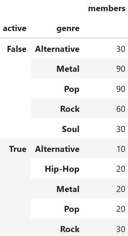
Using this DataFrame, calculate the total variation distance (TVD)
between the "genre" distribution of active bands and the
"genre" distribution of inactive bands. Give your answer as
an exact decimal or simplified fraction.
Answer:
0.3
Solution:
To calculate TVD, we first convert the genre counts into proportions separately for active and inactive bands. We then find the absolute difference between the two proportions for each genre, add these differences, and divide the sum by 2. Using the values in the DataFrame gives a TVD of \boxed{0.3}, indicating that the two genre distributions differ by a total variation distance of 0.3.
Suppose you randomly draw one band uniformly from bands.
You are told that this band is not a rock band. What is
the conditional probability that the band is active? Give your answer as
an exact decimal or simplified fraction.
Answer:
\frac{7}{31}
Solution:
Since we know the selected band is not a rock band, we restrict our attention to the 310 non-rock bands. Of these, 70 are active, so the conditional probability is the number of active non-rock bands divided by the total number of non-rock bands. Therefore, P(\text{Active} \mid \text{Not Rock}) = \frac{70}{310} = \boxed{\frac{7}{31}}.