← return to practice.dsc10.com
Instructor(s): Sam Lau
This exam was administered in-person. The exam was closed-note, except students were allowed 2 pages of hand-written pages of notes and provided a copy of the DSC 10 Reference Sheet. No calculators were allowed. Students had 3 hours to take this exam.
Note (groupby / pandas 2.0): Pandas 2.0+ no longer
silently drops columns that can’t be aggregated after a
groupby, so code written for older pandas may behave
differently or raise errors. In these practice materials we use
.get() to select the column(s) we want after
.groupby(...).mean() (or other aggregations) so that our
solutions run on current pandas. On real exams you will not be penalized
for omitting .get() when the old behavior would have
produced the same answer.
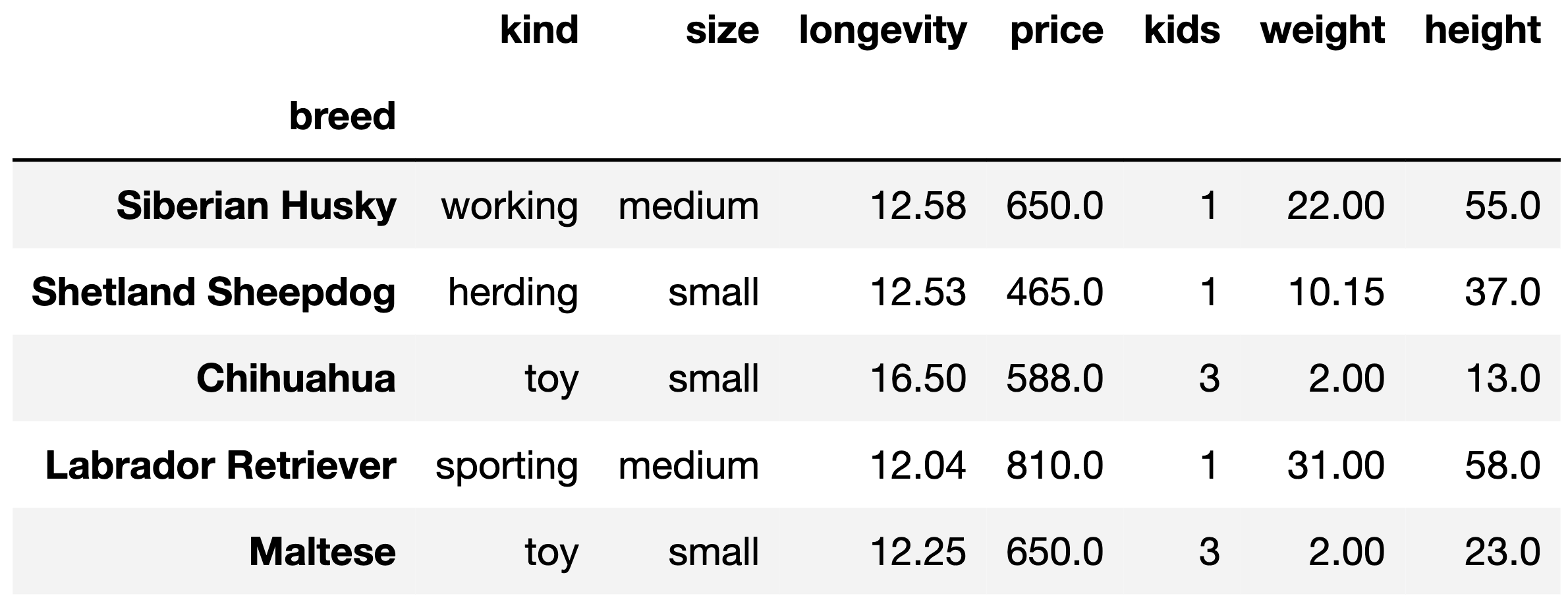
The American Kennel Club (AKC) organizes information about dog
breeds. We’ve loaded their dataset into a DataFrame called
df. The index of df contains the dog breed
names as str values.
The columns are:
'kind' (str): the kind of dog (herding, hound, toy,
etc.). There are six total kinds.'size' (str): small, medium, or large.'longevity' (float): typical lifetime (years).'price' (float): average purchase price (dollars).'kids' (int): suitability for children. A value of
1 means high suitability, 2 means medium, and
3 means low.'weight' (float): typical weight (kg).'height' (float): typical height (cm).The rows of df are arranged in no particular
order. The first five rows of df are shown below
(though df has many more rows than
pictured here).
Assume: - We have already run import babypandas as bpd
and import numpy as np.
Throughout this exam, we will refer to
df repeatedly.
Choose the best visualization to answer each of the following questions.
What kinds of dogs cost the most?
Bar plot
Scatter plot
Histogram
None
Answer: Bar plot
Here, there is a categorical variable (the breed of the dog) and a quantitative variable (the price of the dog). A bar plot is most suitable for this scenario when trying to compare quantitative values accross different categorical values. A scatter plot or histogram wouldn’t be appropriate here since both of those charts typically aim to visualize a comparison between two quantitative variables.
The average score on this problem was 89%.
Do toy dogs have smaller 'size' values than other
dogs?
Bar plot
Scatter plot
Histogram
None
Answer: None of the above
We are comparing two categorical variables ('size' and
'kind'). None of the graphs here are suitable for this
scenario since bar plots are used to compare a categorical variable
against a quantitative variable, while scatter plots and histograms
compare a quantitative variable against quantitative variable.
The average score on this problem was 26%.
Is there a linear relationship between weight and height?
Bar plot
Scatter plot
Histogram
None
Answer: Scatter plot
When looking for a relationship between two continuous quantitative variables, a scatter plot is the most appropriate graph here since the primary use of a scatter plot is to observe the relationship between two numerical variables. A bar chart isn’t suitable since we have two quantitative variables, while a bar chart visualizes a quantitative variable and a categorical variable. A histogram isn’t suitable since it’s typically used to show the frequency of each interval (in other words, the distribution of a numerical variable).
The average score on this problem was 100%.
Do dogs that are highly suitable for children weigh more?
Bar plot
Scatter plot
Histogram
None
Answer: Bar plot
We’re comparing a categorical variable (dog suitability for children) with a quantitative varible (weight). A bar plot is most approriate when comparing a categorical variable against a quantitative variable. Both scatter plot and histogram aim to compare a quantitative variable against another quantitative variable.
The average score on this problem was 40%.
The following code computes the breed of the cheapest toy dog.
df[__(a)__].__(b)__.__(c)__Fill in part (a).
Answer: df.get('kind') == 'toy'
To find the cheapest toy dog, we can start by narrowing down our
dataframe to only include dogs that are of kind toy. We do this by
constructing the following boolean condition:
df.get('kind') == 'toy', which will check whether a dog is
of kind toy (i.e. whether or not a given row’s 'kind' value
is equal to 'toy'). As a result,
df[df.get('kind') == 'toy'] will retrieve all rows for
which the 'kind' column is equal to 'toy'.
The average score on this problem was 91%.
Fill in part (b).
Answer: .sort_values('price')
Next, we can sort the resulting dataframe by price, which will make
the minimum price (i.e. the cheapest toy dog) easily accessible to us
later on. To sort the dataframe, simply use .sort_values(),
with parameter 'price' as follows:
.sort_values('price')
The average score on this problem was 86%.
Which of the following can fill in blank (c)? Select all that apply.
loc[0]
iloc[0]
index[0]
min()
Answer: index[0]
loc[0]: loc retrieves an element by the
row label, which in this case is by 'breed', not by index
value. Furthermore, loc actually returns the entire row,
which is not what we are looking for. (Note that we are trying to find
the singular 'breed' of the cheapest toy dog.)iloc[0]: While iloc does retrieve elements
by index position, iloc actually returns the entire row,
which is not what we are looking for.index[0]: Note that since 'breed' is the
index column of our dataframe, and since we have already filtered and
sorted the dataframe, simply taking the 'breed' at index 0,
or index[0] will return the 'breed' of the
cheapest toy dog.min(): min() is a method used to find the
smallest value on a series not a dataframe.
The average score on this problem was 81%.
The following code computes an array containing the unique kinds of dogs that are heavier than 20 kg or taller than 40 cm on average.
foo = df.__(a)__.__(b)__
np.array(foo[__(c)__].__d__)Fill in blank (a).
Answer: groupby('kind')
We start this problem by grouping the dataframe by
'kind' since we’re only interested in whether each unique
'kind' of dog fits some sort of constraint. We don’t quite
perform querying yet since we need to group the DataFrame first. In
other words, we first need to group the DataFrame into each
'kind' before we could apply any sort of boolean
conditionals.
The average score on this problem was 97%.
Fill in blank (b).
Answer: .mean()
After we do .groupby('kind'), we need to apply
.mean() since the problem asks if each unique
'kind' of dog satisfies certain constraints on
average. .mean() calculates the average of each
column of each group which is what we want.
The average score on this problem was 94%.
Fill in blank (c).
Answer:
(foo.get('weight') > 20) | (foo.get('height') > 40)
Once we have grouped the dogs by 'kind' and have
calculated the average stats of each kind of dog, we can do some
querying with two conditionals: foo.get('weight') > 20
gets the kinds of dogs that are heavier than 20 kg on average and
foo.get('height') > 40 gets the kinds of dogs that are
taller than 40 cm on average. We combine these two conditions with the
| operator since we want the kind of dogs that satisfy
either condition.
The average score on this problem was 93%.
Which of the following should fill in blank (d)?
.index
.unique()
.get('kind')
.get(['kind'])
Answer: .index
Note that earlier, we did groupby('kind'), which
automatically sets each unique 'kind' as the index. Since
this is what we want anyways, simply doing .index will give
us all the kinds of dogs that satisfy the given conditions.
The average score on this problem was 94%.
Let’s say that right after blank (b), we added
reset_index(). Now, which of the following should fill in
blank (d)?
.index
.unique()
.get('kind')
.get(['kind'])
Answer: .get('kind')
Now that we have reset the index of the dataframe,
'kind' is once again its own column so we could simply do
.get('kind').
The average score on this problem was 100%.
The sums function takes in an array of numbers and
outputs the cumulative sum for each item in the array. The cumulative
sum for an element is the current element plus the sum of all the
previous elements in the array.
For example:
>>> sums(np.array([1, 2, 3, 4, 5]))
array([1, 3, 6, 10, 15])
>>> sums(np.array([100, 1, 1]))
array([100, 101, 102])
The incomplete definition of sums is shown below.
def sums(arr):
    res = _________
             (a)
    res = np.append(res, arr[0])
    for i in _________:
                (b)
        res = np.append(res, _________)
                                (c)
return resFill in blank (a).
Answer: np.array([]) or
[]
res is the list in which we’ll be storing each
cumulative sum. Thus we start by initializing res to an
empty array or list.
The average score on this problem was 100%.
Fill in blank (b).
Answer: range(1, len(arr)) or
np.arange(1, len(arr))
We’re trying to loop through the indices of arr and
calculate the cumulative sum corresponding to each entry. To access each
index in sequential order, we simply use range() or
np.arange(). However, notice that we have already appended
the first entry of arr to res on line 3 of the
code snippet. (Note that the first entry of arr is the same
as the first cumulative sum.) Thus the lower bound of
range() (or np.arange()) actually starts at 1,
not 0. The upper bound is still len(arr) as usual.
The average score on this problem was 64%.
Fill in blank (c).
Answer: res[i - 1] + arr[i] or
sum(arr[:i + 1])
Looking at the syntax of the problem, the blank we have to fill
essentially requires us to calculate the current cumulative sum, since
the rest of line will already append the blank to res for
us. One way to think of a cumulative sum is to add the “current”
arr element to the previous cumulative sum, since the
previous cumulative sum encapsulates all the previous elements. Because
we have access to both of those values, we can easily represent it as
res[i - 1] + arr[i]. The second answer is more a more
direct approach. Because the cumulative sum is just the sum of all the
previous elements up to the current element, we can directly compute it
with sum(arr[:i + 1])
The average score on this problem was 71%.
Shivani wrote a function called doggos defined as
follows:
def doggos(n, lower, upper):
t = df.sample(n, replace=True).get('longevity')
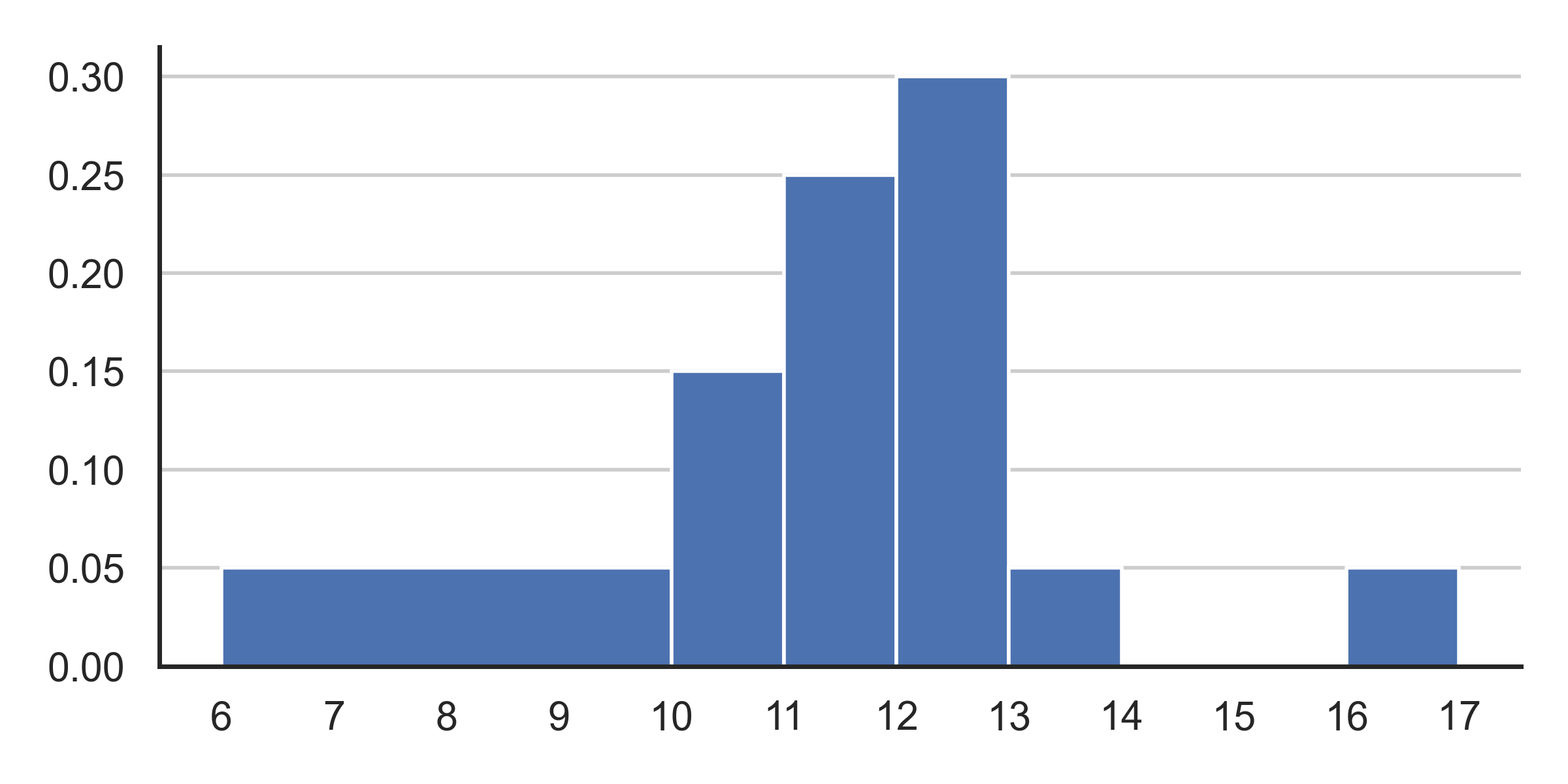
return sum(lower <= t < upper)This plot shows a density histogram of the 'longevity'
column.
Answer each of these questions by either writing a single number in the box or selecting “Not enough information”, but not both. What is the probability that:
doggos(1, 10, 11) == 1 is True?
Answer: 0.15
Let’s first understand the function. The function takes inputs
n, lower, and upper and randomly
takes a sample of n rows with replacement from DataFrame
df, gets column longevity from the sample and
saves it as a Series t. The n entries of
t are randomly generated according to the density histogram
shown in the picture. That is, the probability of a particular value
being generated in Series t for a given entry can be
visualized by the density histogram in the picture.
lower <= t < upper takes t and generates
a Series of boolean values, either True or
False depending on whether the corresponding entry in
t lies within the range. And so
sum(lower <= t < upper) returns the number of entries
in t that lies between the range values. (This is because
True has a value of 1 and False has a value of
0, so summing Booleans is a quick way to count how many
True there are.)
Now part a is just asking for the probability that we’ll draw a
longevity value (given that n is
1, so we only draw one longevity value)
between 10 and 11 given the density plot. Note that the probability of a
bar is given by the width of the bar multiplied by the height. Now
looking at the bar with bin of range 10 to 11, we can see that the
probability is just (11-10) * 0.15 = 1 * 0.15
= 0.15.
The average score on this problem was 86%.
doggos(2, 0, 12) == 2 is True?
Answer: 0.36
Part b is essentially asking us: What is the probability that after
drawing two longevity values according to the density plot,
both of them will lie in between 0 and 12?
Let’s first start by considering the probability of drawing 1
longevity value that lies between 0 and
12. This is simply just the sum of the areas of the three
bars of range 6-10, 10-11, and 11-12, which is just (4*0.05) + (1*0.15) + (1*0.25) = 0.6
Now because we draw each value independently from one another, we simply square this probability which gives us an answer of 0.6*0.6 = 0.36
The average score on this problem was 81%.
doggos(2, 13, 20) > 0 is True?
Answer: 0.19
Part c is essentially asking us: What is the probability that after
drawing two longevity values according to the density plot,
at least one of them will lie in between 12 and 20?
While you can directly solve for this probability, a faster method would be to solve for the complementary of this problem. That is, we can solve for the probability that none of them lie in between the given ranges. And once we solve this, we can simply subtract our answer from one, because the only options for this scenario is that either at least one of the values lie in between the range, or neither of the values do.
Again, let’s solve for the probability of drawing 1
longevity value that isn’t between the range. Staying true
to our complementary strategy, this is just 1 minus the probability of
drawing a longevity value that is in the
range, which is just 1 - (1*0.05+1*0.05) =
0.9
Again, because we draw each value independently, squaring this probability gives us the probability that neither of our drawn values are in the range, or 0.9*0.9 = 0.81. Finally, subtracting this from 1 gives us our desired answer or 1 - 0.81 =0.19
The average score on this problem was 66%.
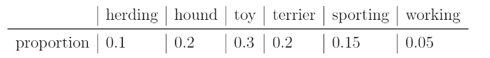
Every year, the American Kennel Club holds a Photo Contest for dogs. Eric wants to know whether toy dogs win disproportionately more often than other kinds of dogs. He has collected a sample of 500 dogs that have won the Photo Contest. In his sample, 200 dogs were toy dogs.
Eric also knows the distribution of dog kinds in the population:
Select all correct statements of the null hypothesis.
The distribution of dogs in the sample is the same as the distribution in the population. Any difference is due to chance.
Every dog in the sample was drawn uniformly at random without replacement from the population.
The number of toy dogs that win is the same as the number of toy dogs in the population.
The proportion of toy dogs that win is the same as the proportion of toy dogs in the population.
The proportion of toy dogs that win is 0.3.
The proportion of toy dogs that win is 0.5.
Answer: Options 4 & 5
A null hypothesis is the hypothesis that there is no significant difference between specified populations, any observed difference being due to sampling or experimental error. Let’s consider what a potential null hypothesis might look like. A potential null hypothesis would be that there is no difference between the win proportion of toy dogs compared to the proportion of toy dogs in the population.
Option 1: We’re not really looking at the distribution of dogs in our sample vs. dogs in our population, rather, we’re looking at whether toy dogs win more than other dogs. In other words, the only factors we’re really consdiering are the proportion of toy dogs to normal dogs, as well as the win percentages of toy dogs to normal dogs; and so the distribution of the population doesn’t really matter. Furthermore, this option makes no reference to win rate of toy dogs.
Option 2: This isn’t really even a null hypothesis, but rather more of a description of a test procedure. This option also makes no attempt to reference to win rate of toy dogs.
Option 3: This statement doesn’t really make sense in that it is illogical to compare the raw number of toy dogs wins to the number of toy dogs in the population, because the number of toy dogs is always at least the number of toy dogs that win.
Option 4: This statement is in line with the null hypothesis.
Option 5: This statement is another potential null hypothesis since the proportion of toy dogs in the population is 0.3.
Option 6: This statement, although similar to Option 5, would not be a null hypothesis because 0.5 has no relevance to any of the relevant proportions. While it’s true that if the proportion of of toy dogs that win is over 0.5, we could maybe infer that toy dogs win the majority of the times; however, the question is not to determine whether toy dogs win most of the times, but rather if toy dogs win a disproportionately high number of times relative to its population size.
The average score on this problem was 83%.
Select the correct statement of the alternative hypothesis.
The model in the null hypothesis underestimates how often toy dogs win.
The model in the null hypothesis overestimates how often toy dogs win.
The distribution of dog kinds in the sample is not the same as the population.
The data were not drawn at random from the population.
Answer: Option 1
The alternative hypothesis is the hypothesis we’re trying to support, which in this case is that toy dogs happen to win more than other dogs.
Option 1: This is in line with our alternative hypothesis, since proving that the null hypothesis underestimates how often toy dogs win means that toy dogs win more than other dogs.
Option 2: This is the opposite of what we’re trying to prove.
Option 3: We don’t really care too much about the distribution of dog kinds, since that doesn’t help us determine toy dog win rates compared to other dogs.
Option 4: Again, we don’t care whether all dogs are chosen according to the probabilities in the null model, instead we care specifically about toy dogs.
The average score on this problem was 67%.
Select all the test statistics that Eric can use to conduct his hypothesis.
The proportion of toy dogs in his sample.
The number of toy dogs in his sample.
The absolute difference of the sample proportion of toy dogs and 0.3.
The absolute difference of the sample proportion of toy dogs and 0.5.
The TVD between his sample and the population.
Answer: Option 1 and Option 2
Option 1: This option is correct. According to our null hypothesis, we’re trying to compare the proportion of toy dogs win rates to the proportion of toy dogs. Thus taking the proportion of toy dogs in Eric’s sample is a perfectly valid test statistic.
Option 2: This option is correct. Since the sample size is fixed at 500, so kowning the count is equivalent to knowing the proportion.
Option 3: This option is incorrect. The absolute difference of the sample proportion of toy dogs and 0.3 doesn’t help us because the absolute difference won’t tell us whether or not the sample proportion of toy dogs is lower than 0.3 or higher than 0.3.
Option 4: This option is incorrect for the same reasoning as above, but also 0.5 isn’t a relevant number anyways.
Option 5: This option is incorrect because TVD measures distance between two categorical distributions, and here we only care about one particular category (not all categories) being the same.
The average score on this problem was 70%.
Eric decides on this test statistic: the proportion of toy dogs minus the proportion of non-toy dogs. What is the observed value of the test statistic?
-0.4
-0.2
0
0.2
0.4
Answer: -0.2
For our given sample, the proportion of toy dogs is \frac{200}{500}=0.4 and the proportion of non-toy dogs is \frac{500-200}{500}=0.6, so 0.4 - 0.6 = -0.2.
The average score on this problem was 74%.
Which snippets of code correctly compute Eric’s test statistic on one
simulated sample under the null hypothesis? Select all that apply. The
result must be stored in the variable stat. Below are the 5
snippets
Snippet 1:
a = np.random.choice([0.3, 0.7])
b = np.random.choice([0.3, 0.7])
stat = a - b
Snippet 2:
a = np.random.choice([0.1, 0.2, 0.3, 0.2, 0.15, 0.05])
stat = a - (1 - a)
Snippet 3:
a = np.random.multinomial(500, [0.1, 0.2, 0.3, 0.2, 0.15, 0.05]) / 500
stat = a[2] - (1 - a[2])
Snippet 4:
a = np.random.multinomial(500, [0.3, 0.7]) / 500
stat = a[0] - (1 - a[0])
Snippet 5:
a = df.sample(500, replace=True)
b = a[a.get("kind") == "toy"].shape[0] / 500
stat = b - (1 - b)
Snippet 1
Snippet 2
Snippet 3
Snippet 4
Snippet 5
Answer: Snippet 3 & Snippet 4
Snippet 1: This is incorrect because
np.random.choice() only chooses values that are either 0.3
or 0.7 which is simply just wrong.
Snippet 2: This is wrong because np.random.choice()
only chooses from the values within the list. From a sanity check it’s
not hard to realize that a should be able to take on more
values than the ones in the list.
Snippet 3: This option is correct. Recall, in
np.random.multinomial(n, [p_1, ..., p_k]), n
is the number of experiments, and [p_1, ..., p_k] is a
sequence of probability. The method returns an array of length k in
which each element contains the number of occurrences of an event, where
the probability of the ith event is p_i. In this snippet,
np.random.multinomial(500, [0.1, 0.2, 0.3, 0.2, 0.15, 0.05])
generates a array of length 6
(len([0.1, 0.2, 0.3, 0.2, 0.15, 0.05])) that contains the
number of occurrences of each kinds of dogs according to the given
distribution (the population distribution). We divide the first line by
500 to convert the number of counts in our resulting array into
proportions. To access the proportion of toy dogs in our sample, we take
the entry with the probability ditribution value of 0.3, which is the
third entry in the array or a[2]. To calculate our test
statistic we take the proportion of toy dogs minus the proportion of
non-toy dogs or a[2] - (1 - a[2])
Snippet 4: This option is correct. This approach is similar to the one above except we’re only considering the probability distribution of toy dogs vs non-toy dogs, which is what we wanted in the first place. The rest of the steps are similar to the ones above.
Snippet 5: Note that df is simple just a dataframe
containing information of the dogs, and may or may not reflect the
population distribution of dogs that participate in the photo
contest.
The average score on this problem was 72%.
After simulating, Eric has an array called sim that
stores his simulated test statistics, and a variable called
obs that stores his observed test statistic.
What should go in the blank to compute the p-value?
np.mean(sim _______ obs) <
<=
==
>=
>
Answer: Option 4: >=
Note that to calculate the p-value we look for test statistics that
are equal to the observed statistic or even further in the direction of
the alternative. In this case, if the proportion of the population of
toy dogs compared to the rest of the dog population was higher than
observed, we’d get a value larger than 0.2, and thus we use
>=.
The average score on this problem was 66%.
Eric’s p-value is 0.03. If his p-value cutoff is 0.01, what does he conclude?
He rejects the null in favor of the alternative.
He accepts the null.
He accepts the aleternative.
He fails to reject the null.
Answer: Option 4: He fails to reject the null
Option 1: Note that since our p-value was greater than 0.01, we fail to reject the null.
Option 2: We can never “accept” the null hypothesis.
Option 3: We didn’t accept the alternative since we failed to reject the null.
Option 4: This option is correct because our p-value was larger than our cutoff.
The average score on this problem was 86%.
Suppose Tiffany has a random sample of dogs. Select the most appropriate technique to answer each of the following questions using Tiffany’s dog sample.
Do small dogs typically live longer than medium and large dogs?
Standard hypothesis test
Permutation test
Bootstrapping
Answer: Option 2: Permutation test.
We have two parameters: dog size and life expectancy. Here if there was no significant statistical difference between the life expectancy of different dog sizes, randomly assigning our sampled life expectancy to each dog should lead us to observe similar observations to the observed statistic. Thus using a permutation test to comapre the two groups makes the most sense. We’re not really trying to estimate a spcecific value so bootstrapping isn’t a good idea here. Also, there’s not really a good way to randomly generate life expectancies so a hypothesis test is not a good idea here.
The average score on this problem was 77%.
Does Tiffany’s sample have an even distribution of dog kinds?
Standard hypothesis test
Permutation test
Bootstrapping
Answer: Option 1: Standard hypothesis test.
We’re not really comparing a variable between two groups, but rather looking at the overall distribution, so Permutation testing wouldn’t work too well here. Again, we’re not really trying to estimate anything here so bootstrapping isn’t a good idea. This leaves us with the Standard Hypothesis Test, which makes sense if we use Total Variation Distance as our test statistic.
The average score on this problem was 51%.
What’s the median weight for herding dogs?
Standard hypothesis test
Permutation test
Bootstrapping
Answer: Option 3: Bootstrapping
Here we’re trying to determine a specific value, which immediately leads us to bootstrapping. The other two tests wouldn’t really make sense in this context.
The average score on this problem was 83%.
Do dogs live longer than 12 years on average?
Standard hypothesis test
Permutation test
Bootstrapping
Answer: Option 3: Bootstrapping
While the wording here might throw us off, we’re really just trying to determine the average life expectancy of dogs, and then see how that compares to 12. This leads us to bootstrapping since we’re trying to determine a specific value. The other two tests wouldn’t really make sense in this context.
The average score on this problem was 43%.
Oren has a random sample of 200 dog prices in an array called
oren. He has also bootstrapped his sample 1,000 times and
stored the mean of each resample in an array called
boots.
In this question, assume that the following code has run:
a = np.mean(oren)
b = np.std(oren)
c = len(oren)What expression best estimates the population’s standard deviation?
b
b / c
b / np.sqrt(c)
b * np.sqrt(c)
Answer: b
The function np.std directly calculated the standard
deviation of array oren. Even though oren is
sample of the population, its standard deviation is still a pretty good
estimate for the standard deviation of the population because it is a
random sample. The other options don’t really make sense in this
context.
The average score on this problem was 57%.
Which expression best estimates the mean of boots?
0
a
(oren - a).mean()
(oren - a) / b
Answer: a
Note that a is equal to the mean of oren,
which is a pretty good estimator of the mean of the overall population
as well as the mean of the distribution of sample means. The other
options don’t really make sense in this context.
The average score on this problem was 89%.
What expression best estimates the standard deviation of
boots?
b
b / c
b / np.sqrt(c)
(a -b) / np.sqrt(c)
Answer: b / np.sqrt(c)
Note that we can use the Central Limit Theorem for this problem which
states that the standard deviation (SD) of the distribution of sample
means is equal to (population SD) / np.sqrt(sample size).
Since the SD of the sample is also the SD of the population in this
case, we can plug our variables in to see that
b / np.sqrt(c) is the answer.
The average score on this problem was 91%.
What is the dog price of $560 in standard units?
(560 - a) / b
(560 - a) / (b / np.sqrt(c))
(a - 560) / (b / np.sqrt(c))}
abs(560 - a) / b
abs(560 - a) / (b / np.sqrt(c))
Answer: (560 - a) / b
To convert a value to standard units, we take the value, subtract the
mean from it, and divide by SD. In this case that is
(560 - a) / b, because a is the mean of our
dog prices sample array and b is the SD of the dog prices
sample array.
The average score on this problem was 80%.
The distribution of boots is normal because of the
Central Limit Theorem.
True
False
Answer: True
True. The central limit theorem states that if you have a population and you take a sufficiently large number of random samples from the population, then the distribution of the sample means will be approximately normally distributed.
The average score on this problem was 91%.
If Oren’s sample was 400 dogs instead of 200, the standard deviation
of boots will…
Increase by a factor of 2
Increase by a factor of \sqrt{2}
Decrease by a factor of 2
Decrease by a factor of \sqrt{2}
None of the above
Answer: Decrease by a factor of \sqrt{2}
Recall that the central limit theorem states that the STD of the
sample distribution is equal to
(population STD) / np.sqrt(sample size). So if we increase
the sample size by a factor of 2, the STD of the sample distribution
will decrease by a factor of \sqrt{2}.
The average score on this problem was 80%.
If Oren took 4000 bootstrap resamples instead of 1000, the standard
deviation of boots will…
Increase by a factor of 4
Increase by a factor of 2
Decrease by a factor of 2
Decrease by a factor of 4
None of the above
Answer: None of the above
Again, from our formula given by the central limit theorem, the
sample STD doesn’t depend on the number of bootstrap resamples so long
as it’s “sufficiently large”. Thus increasing our bootstrap sample from
1000 to 4000 will have no effect on the std of boots
The average score on this problem was 74%.
Write one line of code that evaluates to the right endpoint of a 92% CLT-Based confidence interval for the mean dog price. The following expressions may help:
stats.norm.cdf(1.75) # => 0.96
stats.norm.cdf(1.4) # => 0.92Answer: a + 1.75 * b / np.sqrt(c)
Recall that a 92% confidence interval means an interval that consists
of the middle 92% of the distribution. In other words, we want to “chop”
off 4% from either end of the ditribution. Thus to get the right
endpoint, we want the value corresponding to the 96th percentile in the
mean dog price distribution, or
mean + 1.75 * (SD of population / np.sqrt(sample size) or
a + 1.75 * b / np.sqrt(c) (we divide by
np.sqrt(c) due to the central limit theorem). Note that the
second line of information that was given
stats.norm.cdf(1.4) is irrelavant to this particular
problem.
The average score on this problem was 48%.
Suppose you want to estimate the proportion of UCSD students that love dogs using a survey with a yes/no question. If you poll 400 students, what is the widest possible width for a 95% confidence interval?
0.01
0.05
0.1
0.2
0.5
None of the above
Answer: Option 3: 0.1
Since, we’re looking at a proportion of UCSD students that love dogs,
we’ll set a “yes” vote to a value of 1 and a “no” vote to a value of 0.
(Try to see why this makes the mean of “yes”/“no” votes also the
proportion of “yes” votes). Also by central limit theorem, the
distribution of the sample mean is approximately normal. Now recall that
a 95% confidence interval of a sample mean is given by
[sample mean - 2 * (sample std / np.sqrt(sample size)), sample mean + 2 * (sample std / np.sqrt(sample size))].
As a result, we realize that the width of a 95% confidence interval is
4 * (sample std / np.sqrt(sample size)). Now, the sample
size is already constant, which was given to be 400. However, we can
attempt to maximize the sample std. It’s not hard to see
that the maximum std we could achieve is by recieving an equal number of
yes/no votes (aka 200 of each vote). Calculating the standard deviation
in this case is just 0.5*, and so the widest possible width for a 95%
confidence interval is just 4 * 0.5/np.sqrt(400) which
evaluates to 0.1.
*To make the calculation of the standard deviation faster, try to see why calculating the std of a dataset with 200 1’s and 200 0’s is the same as calculating the std of a data set with only a single 1 and a single 0.
The average score on this problem was 34%.
Sam wants to fit a linear model to predict a dog’s height using its weight.
He first runs the following code:
x = df.get('weight')
y = df.get('height')

def su(vals):
return (vals - vals.mean()) / np.std(vals)Select all of the Python snippets that correctly compute the
correlation coefficient into the variable r.
Snippet 1:
r = (su(x) * su(y)).mean()Snippet 2:
r = su(x * y).mean()Snippet 3:
t = 0
for i in range(len(x)):
    t = t + su(x[i]) * su(y[i])
r = t / len(x)
Snippet 4:
t = np.array([])
for i in range(len(x)):
    t = np.append(t, su(x)[i] * su(y)[i])
r = t.mean()
Snippet 1
Snippet 2
Snippet 3
Snippet 4
Answer: Snippet 1 & 4
Snippet 1: Recall from the reference sheet, the correlation
coefficient is r = (su(x) * su(y)).mean().
Snippet 2: We have to standardize each variable separately so this snippet doesn’t work.
Snippet 3: Note that for this snippet we’re standardizing each
data point within each variable separately, and so we’re not really
standardizing the entire variable correctly. In other words, applying
su(x[i]) to a singular data point is just going to convert
this data point to zero, since we’re only inputting one data point into
su().
Snippet 4: Note that this code is just the same as Snippet 1, except we’re now directly computing the product of each corresponding data points individually. Hence this Snippet works.
The average score on this problem was 81%.
Sam computes the following statistics for his sample:
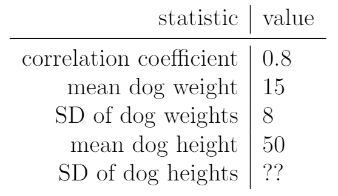
The best-fit line predicts that a dog with a weight of 10 kg has a height of 45 cm.
What is the SD of dog heights?
2
4.5
10
25
45
None of the above
Answer: Option 3: 10
The best fit line in original units are given by
y = mx + b where m = r * (SD of y) / (SD of x)
and b = (mean of y) - m * (mean of x) (refer to reference
sheet). Let c be the STD of y, which we’re trying to find,
then our best fit line is now y = (0.8*c/8)x +
(50-(0.8*c/8)*15). Plugging the two values they gave us into our
best fit line and simplifying gives 45 =
0.1*c*10 + (50 - 1.5*c) which simplifies to 45 = 50 - 0.5*c which gives us an answer of
c = 10.
The average score on this problem was 89%.
Assume that the statistics in part b) still hold. Select all of the statements below that are true. (You don’t need to finish part b) in order to solve this question.)
The relationship between dog weight and height is linear.
The root mean squared error of the best-fit line is smaller than 5.
The best-fit line predicts that a dog that weighs 15 kg will be 50 cm tall.
The best-fit line predicts that a dog that weighs 10 kg will be shorter than 50 cm.
Answer: Option 3 & 4
Option 1: We cannot determine whether two variables are linear simply from a line of best fit. The line of best fit just happens to find the best linear relationship between two varaibles, not whether or not the variables have a linear relationship.
Option 2: To calculate the root mean squared error, we need the actual data points so we can calculate residual values. Seeing that we don’t have access to the data points, we cannot say that the root mean squared error of the best-fit line is smaller than 5.
Option 3: This is true accrding to the problem statement given in part b
Option 4: This is true since we expect there to be a positive correlation between dog height and weight. So dogs that are lighter will also most likely be shorter. (ie a dog that is lighter than 15 kg will most likely be shorter than 50cm)
The average score on this problem was 72%.
Answer the following true/false questions.
Note: This problem is out of scope; it covers material no longer included in the course.
When John Snow took off the handle from the Broad Street pump, the number of cholera deaths decreased. Because of this, he could conclude that cholera was caused by dirty water.
True
False
Answer: False
There are a couple details that the problem fails to convey and that we cannot assume. 1) Do we even know that the pump he removed was the only pump with dirty water? 2) Do we know that people even drank/took water from the Broad Street pump? 3) Do we even know what kinds of people drank from the Broad Street pump? We need to eliminate all confounding factors, otherwise, it might be difficult to identify causality.
The average score on this problem was 91%.
If you get a p-value of 0.009 using a permutation test, you can conclude causality.
True
False
Answer: False
Permutation tests don’t prove causality. Remember, we use the permutation test and calculate a p-value to simply reject a null hypothesis, not to prove the alternative hypothesis.
The average score on this problem was 91%.
df.groupby("kind").mean() will have 5 columns.
True
False
Answer: True
Referring to df at the beginning of the exam, we could
see that 5 of the columns have numerical values as inputs, and thus
df.groupby("kind").mean() will return the mean of these 5
numerical columns
The average score on this problem was 74%.
If the 95% confidence interval for dog price is [650, 900], there is a 95% chance that the population dog price is between $650 and $900.
Answer: False
Recall, what a k% confidence level states is that approximately k% of the time, the intervals you create through this process will contain the true population parameter. In this case, the confidence interval states that approximately 95% of the time, the intervals you create through this process will contain the population dog price. However, it will be false if we state it in the reverse order since our population parameter is already fixed.
The average score on this problem was 66%.
For a given sample, an 90% confidence interval is narrower than a 95% confidence interval.
True
False
Answer: True
The more narrow an interval is, the less confident one is that the intervals one creates will contain the true population parameter.
The average score on this problem was 91%.
If you tried to bootstrap your sample 1,000 times but accidentally sampled without replacement, the standard deviation of your test statistics is always equal to 0.
True
False
Answer: True
Note that bootstrapping form a sample without replacement just means that we’re drawing the same sample over and over again. So the resulting test statistic will be the same between each sample, and thus the std of the test statistic is 0.
The average score on this problem was 86%.
You run a permutation test and store 500 simulated test statistics in
an array called stats. You can construct a 95% confidence
interval by finding the 2.5th and 97.5th percentiles of
stats.
True
False
Answer: False
False, to calculate a 95 percent confidence interval, we use bootstrapping to add variation to our samples.
The average score on this problem was 40%.
The distribution of sample proportions is roughly normal for large samples because of the Central Limit Theorem.
True
False
Answer: True
This is just the definition of Central Limit Theorem.
The average score on this problem was 43%.
Note: This problem is out of scope; it covers material no longer included in the course.
The 20th percentile of the sequence [10, 30, 50, 40, 9, 70] is 30.
True
False
Answer: False
Recall, we find the pth percentile in 4 steps:
Sort the collection in increasing order. [9, 10, 30, 40, 50, 70]
Define h to be p\% of n: h = \frac p{100} \cdot n h = \frac {20}{100} \cdot 6 = 1.2
If h is an integer, define k = h. Otherwise, let k be the smallest integer greater than h. Since h (which is 1.2) is not an integer, so k is 2
Take the kth element of the sorted collection (start counting from 1, not 0). Since 10 has an ordinal rank of 2 in the data set, the 20th percentile value of the data set is 10, not 30.
The average score on this problem was 66%.
Chebyshev’s inequality implies that we can always create a 96% confidence interval from a bootstrap distribution using the mean of the distribution plus or minus 5 standard deviations.
Answer: True
By Chebyshev’s theorem, at least 1 - 1 / z^2 of the data
is within z STD of the mean. Thus at least
1 - 1 / 5^2 = 0.96 of the data is within 5 STD of the
mean.
The average score on this problem was 51%.