← return to practice.dsc10.com
Instructor(s): Janine Tiefenbruck
This exam was administered remotely via Gradescope. The exam was open-internet, and students were able to use Jupyter Notebooks. They had 3 hours to work on it.
Note (groupby / pandas 2.0): Pandas 2.0+ no longer
silently drops columns that can’t be aggregated after a
groupby, so code written for older pandas may behave
differently or raise errors. In these practice materials we use
.get() to select the column(s) we want after
.groupby(...).mean() (or other aggregations) so that our
solutions run on current pandas. On real exams you will not be penalized
for omitting .get() when the old behavior would have
produced the same answer.
One way to use np.arange to produce the sequence
[2, 6, 10, 14] is np.arange(2, 15, 4). This
gives three inputs to np.arange.
Fill in the blanks below to show a different way to produce the same
sequence, this time using only one input to np.arange. Each blank below
must be filled in with a single number only, and the final result,
x*np.arange(y)+z, must produce the sequence
[2, 6, 10, 14].
Using x*np.arange(y)+z fill in the missing values:
x = _
y = _
z = _
Answer:
x = 4, y = 4, z = 2
The question states that we are trying to create the sequence
[2, 6, 10, 14] by filling in the blanks for the statement
x*np.arange(y)+z. If we look at the sequence we are
attempting to derive, we can see that each step in the sequence
increments by 4. Similarly, we can see that the sequence begins at 2. We
know that passing an argument by itself in np.arange will
increment up to that number (for example np.arange(4) will
produce the sequence [0,1,2,3]). Knowing this, we can
create this sequence by setting y to 4. Attempting to reach the desired
sequence of [2, 6, 10, 14] from [0, 1, 2, 3]
we can multiply each number by 4 by setting x to 4 and instantiate the
sequence at 2 by setting z as 2.
The average score on this problem was 96%.
The command .set_index can take as input one column, to
be used as the index, or a sequence of columns to be used as a nested
index (sometimes called a MultiIndex). A MultiIndex is the default
behavior of the dataframe returned by .groupby with multiple
columns.
You are given a dataframe called restaurants that contains information on a variety of local restaurants’ daily number of customers and daily income. There is a row for each restaurant for each date in a given five-year time period.
The columns of restaurants are 'name'
(str), 'year' (int),
'month' (int), 'day'
(int), 'num_diners' (int), and
'income' (float).
Assume that in our data set, there are not two different restaurants that go by the same name (chain restaurants, for example).
Which of the following would be the best way to set the index for this dataset?
restaurants.set_index('name')
restaurants.set_index(['year', 'month', 'day'])
restaurants.set_index(['name', 'year', 'month', 'day'])
Answer:
restaurants.set_index(['name', 'year', 'month', 'day'])
The correct answer is to create an index with the
'name', 'year', ‘month’, and
‘day’ columns. The question provides that there is a row
for each restaurant for each data in the five year span. Therefore, we
are interested in the granularity of a specific day (the day, the month,
and the year). In order to have this information available in this
index, we must set the index to be a multi index with columns
['name', 'year', 'month', 'day']. Looking at the other
options, simply looking at the 'name' column would not
account for the fact the dataframe contains daily data on customers and
income for each restaurant. Similarly, the second option of
['name', 'month', 'day'] would not account for the fact
that the data comes in a five year span so there will naturally be five
overlaps (one for each year) for each unique date that must be accounted
for.
The average score on this problem was 53%.
If we merge a table with n rows with a table with
m rows, how many rows does the resulting table have?
n
m
max(m,n)
m * n
not enough information to tell
Answer: not enough information to tell
The question does not provide enough information to know the resulting table size with certainty. When merging two tables together, the tables can be merged with a inner, left, right, and outer join. Each of these joins will produce a different amount of rows. Since the question does not provide the type of join, it is impossible to tell the resulting table size.
The average score on this problem was 74%.
You sample from a population by assigning each element of the
population a number starting with 1. You include element 1 in your
sample. Then you generate a random number, n, between 2 and
5, inclusive, and you take every nth element after element
1 to be in your sample. For example, if you select n=2,
then your sample will be elements 1, 3, 5, 7, and so
on.
True or False: Before the sample is drawn, you can calculate the probability of selecting each subset of the population.
Answer: True
The answer is true since someone can easily sketch each sample to view the probability of selecting a certain subset. For example, when n = 2 we know the elements are 1, 3, 5, 7, and so on. Similarly we know this information for n = 3, 4 and 5. Using this information we could calculate the probability of selecting a subset.
The average score on this problem was 97%.
True or False: Each subset of the population is equally likely to be selected.
Answer: False
No, each subset of the population is not equally likely to be selected since the element assigned as element 1 will always be selected due to the way sampling is conducted as defined in the question. That is, the question says we always include element one in the sample which will over represent it in samples as compared to other parts of the population.
The average score on this problem was 46%.
You are given a table called books that contains columns
'author' (str), 'title'
(str), 'num_chapters' (int), and
'publication_year' (int).
What will be the output of the following code?
books.groupby(“publication_year”).mean().shape[1]
1
2
3
4
Answer: 1
The output will return 1. Notice that the final function call is to
.shape[1]. We know that .shape[1] is a call to
see how many columns are in the resulting data frame. When we group by
publication year, there is only one column that will be aggregated by
the groupby call (which is the 'num_chapters' column). The
other columns are string, and therefore, will not be aggregated in the
groupby call (since you can’t take the mean of a string). Consequently
.shape[1] will only result one column for the mean of the
'num_chapters' column.
The average score on this problem was 67%.
Which of the following strategies would work to compute the absolute difference in the average number of chapters per book for authors “Dean Koontz” and “Charles Dickens”?
group by 'author', aggregate with .mean(),
use get on 'num_chapters' column compute the
absolute value of the difference between
iloc["Charles Dickens"] and
iloc["Dean Koontz"]
do two queries to get two separate tables (one for each of “Dean
Koontz” and “Charles Dickens”), use get on the
'num_chapters' column of each table, use the Series method
.mean() on each, compute the absolute value of the
difference in these two means
group by both 'author' and 'title',
aggregate with .mean(), use get on
'num_chapters' column, use loc twice to find
values in that column corresponding to “Dean Koontz” and “Charles
Dickens”, compute the absolute value of the difference in these two
values
query using a compound condition to get all books corresponding to
“Dean Koontz” or “Charles Dickens”, group by 'author',
aggregate with .mean(), compute absolute value of the
difference in index[0] and index[1]
Answer: do two queries to get two separate tables
(one for each of “Dean Koontz” and “Charles Dickens”), use
get on the 'num_chapters' column of each
table, use the Series method .mean() on each, compute the
absolute value of the difference in these two means
Logically, we want to somehow separate data for author “Dean Koontz”
and “Charles Dickens”. (If we don’t we’ll be taking a mean that includes
the chapters of books from both authors.) To achieve this separation, we
can create two separate tables with a query that specifies a value on
the 'author' column. Now having two separate tables, we can
aggregate on the 'num_chapters' (the column of interest).
To get the 'num_chapters' column we can use the
get method. To actually acquire the mean of the
'num_chapters' column we can evoke the .mean()
call.
The average score on this problem was 80%.
Which of the following will produce the same value as the total number of books in the table?
books.groupby('Title').count().shape[0]
books.groupby('Author').count().shape[0]
books.groupby(['Author, 'Title']).count().shape[0]
Answer:
books.groupby(['Author, 'Title']).count().shape[0]
The key in this question is to understand that different authors can
create books with the same name. The first two options check for each
unique book title (the first response) and check for each unique other
(the second response). To ensure we have all unique author and title
pairs we must group based on both 'Author' and
'Title'. To actually get the number of rows we can take
.shape[0].
The average score on this problem was 56%.
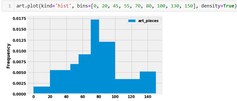
Suppose you have a dataset of 29 art galleries that includes the number of pieces of art in each gallery.
A histogram of the number of art pieces in each gallery, as well as the code that generated it, is shown below.
How many galleries have at least 80 but less than 100 art pieces? Input your answer below. Make sure your answer is an integer and does not include any text or symbols.
Answer: 7
Through looking at the graph we can find the total number of art galleries by taking 0.012 (height of bin) * 20 (the size of the bin) * 29 (total number of art galleries). This will yield an anwser of 6.96 which should be rounded to the nearest integer (7).
The average score on this problem was 94%.
If we added to our dataset two more art galleries, each containing 24
pieces of art, and plotted the histogram again for the larger dataset,
what would be the height of the bin [20,45)? Input your
answer as a number rounded to six decimal places.
Answer: 0.007742
Taking the area of the bin [20,45] we can find the
number of art galleries already within this bin 0.0055 * 25 = 0.1375
(estimation based on the visualization). To find the number take this
proportion x the total number of art galleries. 0.1375 * 29 = about 4
art galleries. If we add two art galleries to this total we get 4 art
galleries in the [20,45] bin to get 6 art galleries. To
find the frequency of 6 art galleries to the entire data set we can take
6/31. Note that the question asks for the height of the bin.
Therefore, we can take (6/31) / 25 due to the size of the bin which will
give an answer of 0.007742 upon rounding to six decimal places.
The average score on this problem was 66%.
Assume df is a DataFrame with distinct rows. Which of
the following best describes df.sample(10)?
an array of length 10, where some of the entries might be the same
an array of length 10, where no two entries can be the same
a DataFrame with 10 rows, where some of the rows might be the same
a DataFrame with 10 rows, where no two rows can be the same
Answer: a DataFrame with 10 rows, where no two rows can be the same
Looking at the documentation for .sample() we can see
that it accepts a few arguments. The first argument specifies the number
of rows (which is why we specify 10). The next argument is a boolean
that specifies if the sampling happens with or without replacement. By
default, the sampling will occur without replacement (which happens in
this question since no argument is specified so the default is evoked).
Looking at the return, we can see that since we are sampling a
dataframe, a dataframe will also be returned which is why a DataFrame
with 10 rows, where no two rows can be the same is correct.
The average score on this problem was 94%.
True or False: If you roll two dice, the probability of rolling two fives is the same as the probability of rolling a six and a three.
Answer: False
The probability of rolling two fives can be found with 1/6 * 1/6 = 1/36. The probability of rolling a six and a three can be found with 2/6 (can roll either a 3 or 6) * 1/6 (roll a different side from 3 or 6, depending on what you rolled first) = 1/18. Therefore, the probabilities are not the same.
The average score on this problem was 33%.
Suppose you do an experiment in which you do some random process 500 times and calculate the value of some statistic, which is a count of how many times a certain phenomenon occurred out of the 500 trials. You repeat the experiment 10,000 times and draw a histogram of the 10,000 statistics.
Is this histogram a probability histogram or an empirical histogram?
probability histogram
empirical histogram
Answer: empirical histogram
Empirical histograms refer to distributions of observed data. Since the question at hand is conducting an experiment and creating a histogram of observed data from these trials the correct anwser is an empirical histogram.
The average score on this problem was 90%.
If you instead repeat the experiment 100,000 times, how will the histogram change?
it will become wider
it will become narrower
it will barely change at all
Answer: it will barely change at all
Doing more of an experiment will barely change the histogram. The parameter we are trying to estimate through our experiment is some statistic. The number of experiments has no effect on the histograms distribution since the value of some statistic is not becoming more random.
The average score on this problem was 57%.
For each experiment, if you instead do the random process 5,000 times, how will the histogram change?
it will become wider
it will become narrower
it will barely change at all
Answer: it will become wider
By increasing the number of random process we increase the possible
range of values from 500 to 5000. The statistic being calculated is the
count of how many times a phenomenon occurs. If the number of random
process increases 10x the statistic can now take values ranging from
[0, 5000] instead of [0, 500] which will
clearly make the histogram width wider (due to the wider range of values
it can take).
The average score on this problem was 39%.
Give an example of a dataset and a question you would want to answer about that dataset which you could answer by performing a permutation test (also known as an A/B test).
Creative responses that are different than ones we’ve already seen in this class will earn the most credit.
Answer: Responses vary. For this question we looked for creative responses. One good example includes
A dataset about prisoners in the US with the sentence times, race, and crime. Do White people who commit homicide get shorter sentence times than Black people who commit homicide? We can clearly perform an A/B test to compare black and white populations as they correlated to shorter sentence times.
The average score on this problem was 93%.
Suppose you draw a sample of size 100 from a population with mean 50 and standard deviation 15. What is the probability that your sample has a mean between 50 and 53? Input the probability below, as a number between 0 and 1, rounded to two decimal places.
Answer: 0.48
This problem is testing our understanding of the Central Limit Theorem and normal distributions. Recall, the Central Limit Theorem tells us that the distribution of the sample mean is roughly normal, with the following characteristics:
\begin{align*} \text{Mean of Distribution of Possible Sample Means} &= \text{Population Mean} = 50 \\ \text{SD of Distribution of Possible Sample Means} &= \frac{\text{Population SD}}{\sqrt{\text{Sample Size}}} = \frac{15}{\sqrt{100}} = 1.5 \end{align*}
Given this information, it may be easier to express the problem as “We draw a value from a normal distribution with mean 50 and SD 1.5. What is the probability that the value is between 50 and 53?” Note that this probability is equal to the proportion of values between 50 and 53 in a normal distribution whose mean is 50 and 1.5 (since probabilities can be thought of as proportions).
In class, we typically worked with the standard normal distribution, in which the mean was 0, the SD was 1, and the x-axis represented values in standard units. Let’s convert the quantities of interest in this problem to standard units, keeping in mind that the mean and SD we’re using now are the mean and SD of the distribution of possible sample means, not of the population.
Now, our problem boils down to finding the proportion of values in a standard normal distribution that are between 0 and 2, or the proportion of values in a normal distribution that are in the interval [\text{mean}, \text{mean} + 2 \text{ SDs}].
From class, we know that in a normal distribution, roughly 95% of values are within 2 standard deviations of the mean, i.e. the proportion of values in the interval [\text{mean} - 2 \text{ SDs}, \text{mean} + 2 \text{ SDs}] is 0.95.
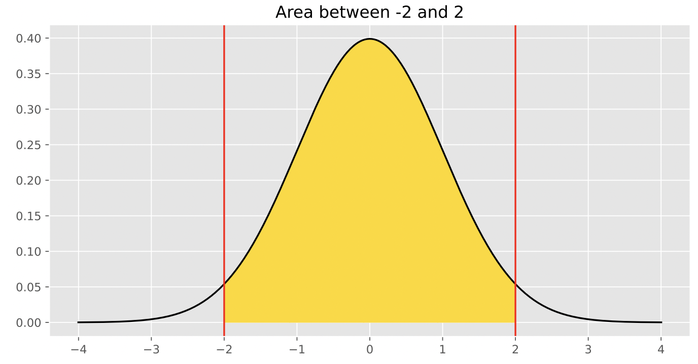
Since the normal distribution is symmetric about the mean, half of the values in this interval are to the right of the mean, and half are to the left. This means that the proportion of values in the interval [\text{mean}, \text{mean} + 2 \text{ SDs}] is \frac{0.95}{2} = 0.475, which rounds to 0.48, and thus the desired result is 0.48.
The average score on this problem was 48%.
You need to estimate the proportion of American adults who want to be vaccinated against Covid-19. You plan to survey a random sample of American adults, and use the proportion of adults in your sample who want to be vaccinated as your estimate for the true proportion in the population. Your estimate must be within 0.04 of the true proportion, 95% of the time. Using the fact that the standard deviation of any dataset of 0’s and 1’s is no more than 0.5, calculate the minimum number of people you would need to survey. Input your answer below, as an integer.
Answer: 625
Note: Before reviewing these solutions, it’s highly recommended to revisit the lecture on “Choosing Sample Sizes,” since this problem follows the main example from that lecture almost exactly.
While this solution is long, keep in mind from the start that our goal is to solve for the smallest sample size necessary to create a confidence interval that achieves certain criteria.
The Central Limit Theorem tells us that the distribution of the sample mean is roughly normal, regardless of the distribution of the population from which the samples are drawn. At first, it may not be clear how the Central Limit Theorem is relevant, but remember that proportions are means too – for instance, the proportion of adults who want to be vaccinated is equal to the mean of a collection of 1s and 0s, where we have a 1 for each adult that wants to be vaccinated and a 0 for each adult who doesn’t want to be vaccinated. What this means (😉) is that the Central Limit Theorem applies to the distribution of the sample proportion, so we can use it here too.
Not only do we know that the distribution of sample proportions is roughly normal, but we know its mean and standard deviation, too:
\begin{align*} \text{Mean of Distribution of Possible Sample Means} &= \text{Population Mean} = \text{Population Proportion} \\ \text{SD of Distribution of Possible Sample Means} &= \frac{\text{Population SD}}{\sqrt{\text{Sample Size}}} \end{align*}
Using this information, we can create a 95% confidence interval for the population proportion, using the fact that in a normal distribution, roughly 95% of values are within 2 standard deviations of the mean:
\left[ \text{Population Proportion} - 2 \cdot \frac{\text{Population SD}}{\sqrt{\text{Sample Size}}}, \: \text{Population Proportion} + 2 \cdot \frac{\text{Population SD}}{\sqrt{\text{Sample Size}}} \right]
However, this interval depends on the population proportion (mean) and SD, which we don’t know. (If we did know these parameters, there would be no need to collect a sample!) Instead, we’ll use the sample proportion and SD as rough estimates:
\left[ \text{Sample Proportion} - 2 \cdot \frac{\text{Sample SD}}{\sqrt{\text{Sample Size}}}, \: \text{Sample Proportion} + 2 \cdot \frac{\text{Sample SD}}{\sqrt{\text{Sample Size}}} \right]
Note that the width of this interval – that is, its right endpoint minus its left endpoint – is: \text{width} = 4 \cdot \frac{\text{Sample SD}}{\sqrt{\text{Sample Size}}}
In the problem, we’re told that we want our interval to be accurate to within 0.04, which is equivalent to wanting the width of our interval to be less than or equal to 0.08 (since the interval extends the same amount above and below the sample proportion). As such, we need to pick the smallest sample size necessary such that:
\text{width} = 4 \cdot \frac{\text{Sample SD}}{\sqrt{\text{Sample Size}}} \leq 0.08
We can re-arrange the inequality above to solve for our sample’s size:
\begin{align*} 4 \cdot \frac{\text{Sample SD}}{\sqrt{\text{Sample Size}}} &\leq 0.08 \\ \frac{\text{Sample SD}}{\sqrt{\text{Sample Size}}} &\leq 0.02 \\ \frac{1}{\sqrt{\text{Sample Size}}} &\leq \frac{0.02}{\text{Sample SD}} \\ \frac{\text{Sample SD}}{0.02} &\leq \sqrt{\text{Sample Size}} \\ \left( \frac{\text{Sample SD}}{0.02} \right)^2 &\leq \text{Sample Size} \end{align*}
All we now need to do is pick the smallest sample size that satisfies the above inequality. But there’s an issue – we don’t know what our sample SD is, because we haven’t collected our sample! Notice that in the inequality above, as the sample SD increases, so does the minimum necessary sample size. In order to ensure we don’t collect too small of a sample (which would result in the width of our confidence interval being larger than desired), we can use an upper bound for the SD of our sample. In the problem, we’re told that the largest possible SD of a sample of 0s and 1s is 0.5 – this means that if we replace our sample SD with 0.5, we will find a sample size such that the width of our confidence interval is guaranteed to be less than or equal to 0.08. This sample size may be larger than necessary, but that’s better than it being smaller than necessary.
By substituting 0.5 for the sample SD in the last inequality above, we get
\begin{align*} \left( \frac{\text{Sample SD}}{0.02} \right)^2 &\leq \text{Sample Size} \\\ \left( \frac{0.5}{0.02} \right)^2 &\leq \text{Sample Size} \\ 25^2 &\leq \text{Sample Size} \implies \text{Sample Size} \geq 625 \end{align*}
We need to pick the smallest possible sample size that is greater than or equal to 625; that’s just 625.
The average score on this problem was 40%.
Rank these three students in ascending order of their exam performance relative to their classmates.
Hector, Clara, Vivek
Vivek, Hector, Clara
Clara, Hector, Vivek
Vivek, Clara, Hector
Answer: Vivek, Hector, Clara
To compare Vivek, Hector, and Clara’s relative performance we want to compare their Z scores to handle standardization. For Vivek, his Z score is (83-75) / 6 = 4/3. For Hector, his score is (77-70) / 5 = 7/5. For Clara, her score is (80-75) / 3 = 5/3. Ranking these, 5/3 > 7/5 > 4/3 which yields the result of Vivek, Hector, Clara.
The average score on this problem was 76%.
The data visualization below shows all Olympic gold medals for women’s gymnastics, broken down by the age of the gymnast.
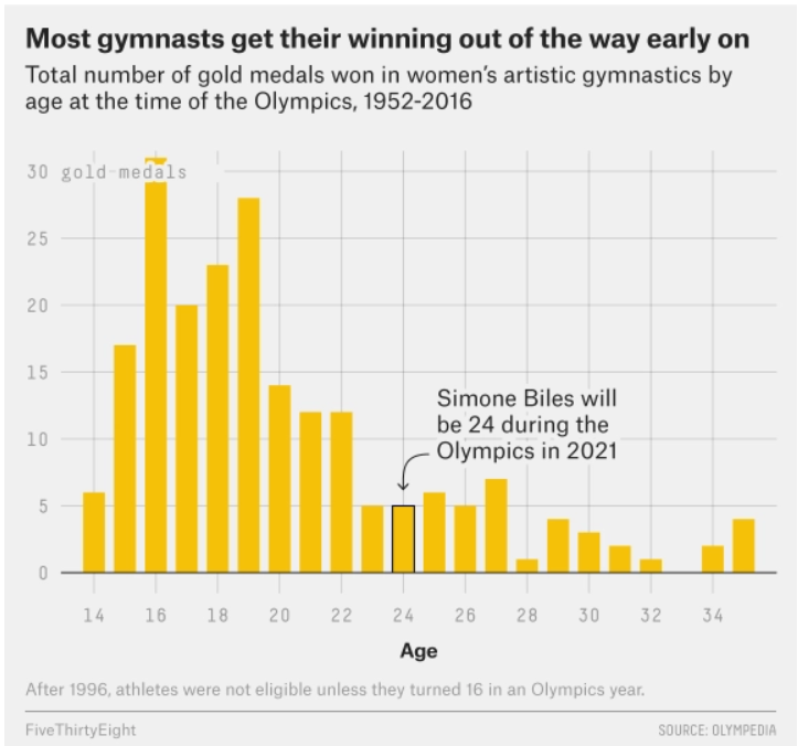
Based on this data, rank the following three quantities in ascending order: the median age at which gold medals are earned, the mean age at which gold medals are earned, the standard deviation of the age at which gold medals are earned.
mean, median, SD
median, mean, SD
SD, mean, median
SD, median, mean
Answer: SD, median, mean
The standard deviation will clearly be the smallest of the three
values as most of the data is encompassed between the range of
[14-26]. Intuitively, the standard deviation will have to
be about a third of this range which is around 4 (though this is not the
exact standard deviation, but is clearly much less than the mean and
median with values closer to 19-25). Comparing the median and mean, it
is important to visualize that this distribution is skewed right. When
the data is skewed right it pulls the mean towards a higher value (as
the higher values naturally make the average higher). Therefore, we know
that the mean will be greater than the median and the ranking is SD,
median, mean.
The average score on this problem was 72%.
Which of the following is larger for this dataset?
the difference between the 50th percentile of ages and the 25th percentile of ages
the difference between the 75th percentile of ages and the 50th percentile of ages
both are the same
Answer: the difference between the 75th percentile of ages and the 50th percentile of ages
Since the distribution is right skewed, the 75th percentile will have a larger difference from the 50th percentile than the 25th percentile. With right skewness, values above the 50th percentile will be more different than those smaller than the 50th percentile (and thus more spread out according to the graph).
The average score on this problem was 78%.
In a board game, whenever it is your turn, you roll a six-sided die
and move that number of spaces. You get 10 turns, and you win the game
if you’ve moved 50 spaces in those 10 turns. Suppose you create a
simulation, based on 10,000 trials, to show the distribution of the
number of spaces moved in 10 turns. Let’s call this distribution
Dist10. You also wonder how the game would be
different if you were allowed 15 turns instead of 10, so you create
another simulation, based on 10,000 trials, to show the distribution of
the number of spaces moved in 15 turns, which we’ll call
Dist15
What can we say about the shapes of Dist10 and Dist15?
both will be roughly normally distributed
only one will be roughly normally distributed
neither will be roughly normally distributed
Answer: both will be roughly normally distributed
By the central limit theorem, both simulations will appear to be roughly normally distributed.
The average score on this problem was 90%.
What can we say about the centers of Dist10 and Dist15?
both will have approximately the same mean
the mean of Dist10 will be smaller than the mean of Dist15
the mean of Dist15 will be smaller than the mean of Dist10
Answer: the mean of Dist10 will be smaller than the mean of Dist15
The distribution which moves in 10 turns will have a smaller mean as there are less turns to move spaces. Therefore, the mean movement from turns will naturally be higher for the distribution with more turns.
The average score on this problem was 83%.
What can we say about the spread of Dist10 and Dist15?
both will have approximately the same standard deviation
the standard deviation of Dist10 will be smaller than the standard deviation of Dist15
the standard deviation of Dist15 will be smaller than the standard deviation of Dist10
Answer: the standard deviation of Dist10 will be smaller than the standard deviation of Dist15
Since taking more turns allows for more possible values, the spread of Dist10 will be smaller than the standard deviation of Dist15. (ie. consider the possible range of values that are attainable for each case)
The average score on this problem was 65%.
True or False: The slope of the regression line, when both variables are measured in standard units, is never more than 1.
Answer: True
Standard units standardize the data into z scores. When converting to Z scores the scale of both the dependent and independent variables are the same, and consequently, the slope can at most increase by 1. Alternatively, according to the reference sheet, the slope of the regression line, when both variables are measured in standard units, is also equal to the correlation coefficient. And by definition, the correlation coefficient can never be greater than 1 (since you can’t have more than a ‘perfect’ correlation).
The average score on this problem was 93%.
True or False: The slope of the regression line, when both variables are measured in original units, is never more than 1.
Answer: False
Original units refers to units as they are. Clearly, regression slopes can be greater than 1 (for example if for every change in 1 unit of x corresponds to a change in 20 units of y the slope will be 20).
The average score on this problem was 96%.
True or False: Suppose that from a sample, you compute a 95% bootstrapped confidence interval for a population parameter to be the interval [L, R]. Then the average of L and R is the mean of the original sample.
Answer: False
A 95% confidence interval indicates we are 95% confident that the true population parameter falls within the interval [L, R]. Note that the problem specifies that the confidence interval is bootstrapped. Since the interval is found using bootstrapping, L and R averaged will not be the mean of the original sample since the mean of the original sample is not what is used in calculating the bootstrapped confidence interval. The bootstrapped confidence interval is created by re-sampling the data with replacement over and over again. Thus, while the interval is typically centered around the sample mean due to the nature of bootstrapping, the average of L and R (the 2.5th and 97.5th percentiles of the distribution of bootstrapped means) may not exactly equal the sample mean, but should be close to it. Additionally, L is the 2.5th percentile of the distribution of bootstrapped means and R is the 97.5th percentile, and these are not necessarily the same distance away from the mean of the sample.
The average score on this problem was 87%.
True or False: Suppose that from a sample, you compute a 95% normal confidence interval for a population parameter to be the interval [L, R]. Then the average of L and R is the mean of the original sample.
Answer: True
True, a 95% confidence interval indicates we are 95% confident that the true population parameter falls within the interval [L, R]. Looking at how a confidence interval is calculated is by adding/ subtracting a confidence level value (z) by the standard error. Since the top and bottom of the interval will be different from the mean by the same amount, the average will be the mean. (For more information, refer to the reference sheet)
The average score on this problem was 68%.
You order 25 large pizzas from your local pizzeria. The pizzeria claims that these pizzas are 16 inches in diameter, but you’re not so sure. You measure each pizza’s diameter and collect a dataset of 25 actual pizza diameters. You want to run a hypothesis test to determine whether the pizzeria’s claim is accurate.
What would your Null Hypothesis be?
What would your Alternative Hypothesis be?
Answer:
Null Hypothesis: The mean pizza diameter at the local pizzeria is 16 inches.
Alternative Hypothesis: The mean pizza diameter at the local pizzeria is not 16 inches.
The null hypothesis is the hypothesis where there is no significant difference from some statement. In this case, the statement of interest is the pizzeria’s claims of pizzas are 16 inches in diameter.
The alternative hypothesis is a statement that contradicts the null hypothesis. In this case this statement is that the mean pizza diameter at the local pizzeria is not 16 inches. (ie. the other option to the null hypothesis)
The average score on this problem was 35%.
What test statistic would you use?
Answer: Mean Pizza Diameter, or other valid statistics such as the (absolute) difference between each pizza’s diameter and 16 (expected value)
Looking at the null and alternative hypothesis we can see we are directly interested in the mean pizza diameter, so it is most likely the best measurement for the test statistic. The main idea is that we somehow want to show the difference in distribution of the pizza diameters.
The average score on this problem was 70%.
Explain how you would do your hypothesis test and how you would draw a conclusion from your results.
Answer: Answers vary, should include the following
Generate confidence interval for population mean (or equivalent) by bootstrapping (or by calculating directly with the sample).
Correctly describe how to reject or fail to reject the null hypothesis (depending on whether interval contains 16, for example).
When conducting the hypothesis test, we first want to create a confidence interval either by using bootstrapping or constructing a 95% confidence interval to understand the true mean diameter of pizzas. The next step is to define the rejection criteria, failing to reject the null if 16 is within the 95% confidence interval (since we believe the true population mean) is within this range with 95% confidence. We will reject the null hypothesis if 16 is not within the 95% confidence interval. Note that this assumes you used true mean diameter of pizzas as your test statistic.
The average score on this problem was 38%.
A restaurant keeps track of each table’s number of people (average 3; standard deviation 1) and the amount of the bill (average $60, standard deviation $12). If the number of people and amount of the bill are linearly associated with correlation 0.8, what is the predicted bill for a table of 5 people? Input your answer below, to the nearest cent. Make sure your answer is just a number and does not include the $ symbol or any text.
Answer: 79.20
To answer this question, first find the z score for a table of 5 people. Z = (5-3)/1 = 2. Now having this Z score, find the price that correlated in the bill distribution by finding the value for 2 standard deviations larger than the mean while also accounting for the correlation between the two variables. This is calculated with mean + ((ZSD) r) which is 60 + ((12 * 2) * 0.8) = 79.20.
Alternatively, we could solve for the regression line and plug our values in according to the reference sheet:
m = (0.8) * (12/1) and b = 60 - (48/5) * 3 (where m is the slope and b is the y-intercept)
Thus plugging the appropriate values in our regression line yields
y = (48/5) * 5 + 60 - (48/5)*3 = 79.2
The average score on this problem was 88%.
From a population with mean 500 and standard deviation 50, you collect a sample of size 100. The sample has mean 400 and standard deviation 40. You bootstrap this sample 10,000 times, collecting 10,000 resample means.
Which of the following is the most accurate description of the mean of the distribution of the 10,000 bootstrapped means?
The mean will be exactly equal to 400.
The mean will be exactly equal to 500.
The mean will be approximately equal to 400.
The mean will be approximately equal to 500.
Answer: The mean will be approximately equal to 400.
The distribution of bootstrapped means’ mean will be approximately 400 since that is the mean of the sample and bootstrapping is taking many samples of the original sample. The mean will not be exactly 400 do to some randomness though it will be very close.
The average score on this problem was 54%.
Which of the following is closest to the standard deviation of the distribution of the 10,000 bootstrapped means?
400
40
4
0.4
Answer: 4
To find the standard deviation of the distribution, we can take the sample standard deviation S divided by the square root of the sample size. From plugging in, we get 40 / 10 = 4.
The average score on this problem was 51%.
Note: This problem is out of scope; it covers material no longer included in the course.
Recall the mathematical definition of percentile and how we calculate it.
By this definition, any percentile between 0 and 100 can be computed for any collection of values and is always an element of the collection. Suppose there are n elements in the collection. To find the pth percentile:
You have a dataset of 7 values, which are
[3, 6, 7, 9, 10, 15, 18]. Using the mathematical definition
of percentile above, find the smallest and largest integer values of p
so that the pth percentile of this dataset corresponds to the value 10.
Input your answers below, as integers between 0 and
100.
Smallest = _
Answer: 58
From the definition provided in the question, we want all values of (p/100) * n which will yield an integer larger than 4, but less than or equal to 5 because we want the 5th element (10) in the dataset. To approach this problem we can find how many percentiles each piece of data falls within by taking 100 / 7 which yields around 14.3. Wanting to find the percentiles for the range of 4 to 5 we can multiple (100/7) by 4 to get our lower bound. (100/7) * 4 = 57.14 which is rounded up to 58 since the 57th percentile belongs to the 4th element while 58 belongs to the fifth element.
The average score on this problem was 73%.
Largest = _
Answer: 71
To find the largest we will take (100/7) * 5 which yields 71.43. We will round down since the 72th percentile belongs to the sixth element in the data set. For more information look at the solution above.
The average score on this problem was 74%.
Are nonfiction books longer than fiction books?
Choose the best data science tool to help you answer this question.
hypothesis testing
permutation (A/B) testing
Central Limit Theorem
regression
Answer: permutation (A/B) testing
The question Are nonfiction books longer than fiction books? is investigating the difference between two underlying populations (nonfiction books and fiction books). A permutation test is the best data science tool when investigating differences between two underlying distributions.
The average score on this problem was 90%.
Do people have more friends as they get older?
Choose the best data science tool to help you answer this question.
hypothesis testing
permutation (A/B) testing
Central Limit Theorem
regression
Answer: regression
The question at hand is investigating two continuous variables (time and number of friends). Regression is the best data science tool as it is dealing with two continuous variables and we can understand correlations between time and the number of friends.
The average score on this problem was 90%.
Does an ice cream shop sell more chocolate or vanilla ice cream cones?
Choose the best data science tool to help you answer this question.
hypothesis testing
permutation (A/B) testing
Central Limit Theorem
regression
Answer: hypothesis testing
The question at hand is dealing with differences between sales of different flavors of ice cream, which is the same thing as the total of ice cream cones sold. We can use hypothesis testing to test our null hypothesis that the count of Vanilla cones sold is higher than Chocolate, and our alternative hypothesis that the count of Chocolate cones sold is more than Vanilla. A permutation test is not suitable here because we are not comparing any numerical quantity associated with each group. A permutation test could be used to answer questions like “Are chocolate ice cream cones more expensive than vanilla ice cream cones?” or “Do chocolate ice cream cones have more calories than vanilla ice cream cones?”, or any other question where you are tracking a number (cost or calories) along with each ice cream cone. In our case, however, we are not tracking a number along with each individual ice cream cone, but instead tracking a total of ice cream cones sold.
An analogy to this hypothesis test can be found in the “fair or unfair coin” problem in Lectures 20 and 21, where our null hypothesis is that the coin is fair and our alternative hypothesis is that the coin is unfair. The “fairness” of the coin is not a numerical quantity that we can track with each individual coin flip, just like how the count of ice cream cones sold is not a numerical quantity that we can track with each individual ice cream cone.
The average score on this problem was 57%.