← return to practice.dsc10.com
Instructor(s): Janine Tiefenbruck
This exam was administered remotely via Gradescope. The exam was open-notes, and students could access any resource including the internet and Jupyter notebooks. Students had 90 minutes to work on it.
Note (groupby / pandas 2.0): Pandas 2.0+ no longer
silently drops columns that can’t be aggregated after a
groupby, so code written for older pandas may behave
differently or raise errors. In these practice materials we use
.get() to select the column(s) we want after
.groupby(...).mean() (or other aggregations) so that our
solutions run on current pandas. On real exams you will not be penalized
for omitting .get() when the old behavior would have
produced the same answer.
Note: This problem is out of scope; it covers material no longer included in the course.
Which of the following questions could not be answered by running a randomized controlled experiment?
Does eating citrus fruits increase the risk of heart disease?
Do exams with integrity pledges have fewer reported cases of academic dishonesty?
Does rewarding students for good grades improve high school graduation rates?
Does drug abuse lead to a shorter life span?
Answer: Does drug abuse lead to a shorter life span?
It would be unethical to try to run a randomized controlled experiment to address the question of whether drug abuse leads to a shorter life span, as this would involve splitting participants into groups and telling one group to abuse drugs. This is problematic because we know drug abuse brings about a host of problems, so we could not ethically ask people to harm themselves.
Notice that the first proposed study, about the impacts of citrus fruits on heart disease, does not involve the same kind of ethical dilemma because we’re not forcing people to do something known to be harmful. A randomized controlled experiment would involve splitting participants into two groups and asking one group to eat citrus fruits, and measuring the heart health of both groups. Since there are no known harmful effects of eating citrus fruits, there is no ethical issue.
Similarly, we could run a randomized controlled trial by giving an exam where some students had to sign an integrity pledge and others didn’t, tracking the number of reported dishonesty cases in each group. Likewise, we could reward some students for good grades and not others, and keep track of high school graduation rates in each group. Neither of these studies would involve knowingly harming people and could reasonably be carried out.
The average score on this problem was 85%.
You are given a DataFrame called sports, indexed by
'Sport' containing one column,
'PlayersPerTeam'. The first few rows of the DataFrame are
shown below:
| Sport | PlayersPerTeam |
|---|---|
| baseball | 9 |
| basketball | 5 |
| field hockey | 11 |
Which of the following evaluates to
'basketball'?
sports.loc[1]
sports.iloc[1]
sports.index[1]
sports.get('Sport').iloc[1]
Answer: sports.index[1]
We are told that the DataFrame is indexed by 'Sport' and
'basketball' is one of the elements of the index. To access
an element of the index, we use .index to extract the index
and square brackets to extract an element at a certain position.
Therefore, sports.index[1] will evaluate to
'basketball'.
The first two answer choices attempt to use .loc or
.iloc directly on a DataFrame. We typically use
.loc or .iloc on a Series that results from
using .get on some column. Although we don’t typically do
it this way, it is possible to use .loc or
.iloc directly on a DataFrame, but doing so would produce
an entire row of the DataFrame. Since we want just one word,
'basketball', the first two answer choices must be
incorrect.
The last answer choice is incorrect because we can’t use
.get with the index, only with a column. The index is never
considered a column.
The average score on this problem was 88%.
The following is a quote from The New York Times’ The Morning newsletter.
As Dr. Ashish Jha, the dean of the Brown University School of Public Health, told me this weekend: “I don’t actually care about infections. I care about hospitalizations and deaths and long-term complications.”
By those measures, all five of the vaccines — from Pfizer, Moderna, AstraZeneca, Novavax and Johnson & Johnson — look extremely good. Of the roughly 75,000 people who have received one of the five in a research trial, not a single person has died from Covid, and only a few people appear to have been hospitalized. None have remained hospitalized 28 days after receiving a shot.
To put that in perspective, it helps to think about what Covid has done so far to a representative group of 75,000 American adults: It has killed roughly 150 of them and sent several hundred more to the hospital. The vaccines reduce those numbers to zero and nearly zero, based on the research trials.
Zero isn’t even the most relevant benchmark. A typical U.S. flu season kills between five and 15 out of every 75,000 adults and hospitalizes more than 100 of them.
Why does the article use a representative group of 75,000 American adults?
Convention. Rates are often given per 75,000 people.
Comparison. It allows for quick comparison against the group of people who got the vaccine in a trial.
Comprehension. Readers should have a sense of the scale of 75,000 people.
Arbitrary. There is no particular reason to use a group of this size.
Answer: Comparison. It allows for quick comparison against the group of people who got the vaccine in a trial.
The purpose of the article is to compare Covid outcomes among two groups of people: the 75,000 people who got the vaccine in a research trial and a representative group of 75,000 American adults. Since 75,000 people got the vaccine in a research trial, we need to compare statistics like number of deaths and hospitalizations to another group of the same size for the comparison to be meaningful.
There is no convention about using 75,000 for rates. This number is used because that’s how many people got the vaccine in a research trial. If a different number of people had been vaccinated in a research trial, the article would have taken that number of adults in their representative comparison group.
75,000 is quite a large number and most people probably don’t have a sense of the scale of 75,000 people. If the goal were comprehension, it would have made more sense to use a smaller number like 100 people.
The number 75,000 is not arbitrary. It was chosen as the size of the representative group specifically to equal the number of people who got the vaccine in a research trial.
The average score on this problem was 91%.
Suppose you are given a DataFrame of employees for a given company.
The DataFrame, called employees, is indexed by
'employee_id' (string) with a column called
'years' (int) that contains the number of years each
employee has worked for the company.
Suppose that the code
employees.sort_values(by='years', ascending=False).index[0]outputs '2476'.
True or False: The number of years that employee 2476 has worked for the company is greater than the number of years that any other employee has worked for the company.
True
False
Answer: False
This is false because there could be other employees who worked at the company equally long as employee 2476.
The code says that when the employees DataFrame is
sorted in descending order of 'years', employee 2476 is in
the first row. There might, however, be a tie among several employees
for their value of 'years'. In that case, employee 2476 may
wind up in the first row of the sorted DataFrame, but we cannot say that
the number of years employee 2476 has worked for the company is greater
than the number of years that any other employee has worked for the
company.
If the statement had said greater than or equal to instead of greater than, the statement would have been true.
The average score on this problem was 29%.
What will be the output of the following code?
employees.assign(start=2021-employees.get('years'))
employees.sort_values(by='start').index.iloc[-1]
the employee id of an employee who has worked there for the most years
the employee id of an employee who has worked there for the fewest years
an error message complaining about iloc[-1]
an error message complaining about something else
Answer: an error message complaining about something else
The problem is that the first line of code does not actually add a
new column to the employees DataFrame because the
expression is not saved. So the second line tries to sort by a column,
'start', that doesn’t exist in the employees
DataFrame and runs into an error when it can’t find a column by that
name.
This code also has a problem with iloc[-1], since
iloc cannot be used on the index, but since the problem
with the missing 'start' column is encountered first, that
will be the error message displayed.
The average score on this problem was 27%.
Suppose df is a DataFrame and b is any
boolean array whose length is the same as the number of rows of
df.
True or False: For any such boolean array b,
df[b].shape[0] is less than or equal to
df.shape[0].
True
False
Answer: True
The brackets in df[b] perform a query, or filter, to
keep only the rows of df for which b has a
True entry. Typically, b will come from some
condition, such as the entry in a certain column of df
equaling a certain value. Regardless, df[b] contains a
subset of the rows of df, and .shape[0] counts
the number of rows, so df[b].shape[0] must be less than or
equal to df.shape[0].
The average score on this problem was 86%.
You are given a DataFrame called books that contains
columns 'author' (string), 'title' (string),
'num_chapters' (int), and 'publication_year'
(int).
Suppose that after doing books.groupby('Author').max(),
one row says
| author | title | num_chapters | publication_year |
|---|---|---|---|
| Charles Dickens | Oliver Twist | 53 | 1838 |
Based on this data, can you conclude that Charles Dickens is the alphabetically last of all author names in this dataset?
Yes
No
Answer: No
When we group by 'Author', all books by the same author
get aggregated together into a single row. The aggregation function is
applied separately to each other column besides the column we’re
grouping by. Since we’re grouping by 'Author' here, the
'Author' column never has the max() function
applied to it. Instead, each unique value in the 'Author'
column becomes a value in the index of the grouped DataFrame. We are
told that the Charles Dickens row is just one row of the output, but we
don’t know anything about the other rows of the output, or the other
authors. We can’t say anything about where Charles Dickens falls when
authors are ordered alphabetically (but it’s probably not last!)
The average score on this problem was 94%.
Based on this data, can you conclude that Charles Dickens wrote Oliver Twist?
Yes
No
Answer: Yes
Grouping by 'Author' collapses all books written by the
same author into a single row. Since we’re applying the
max() function to aggregate these books, we can conclude
that Oliver Twist is alphabetically last among all books in the
books DataFrame written by Charles Dickens. So Charles
Dickens did write Oliver Twist based on this data.
The average score on this problem was 95%.
Based on this data, can you conclude that Oliver Twist has 53 chapters?
Yes
No
Answer: No
The key to this problem is that groupby applies the
aggregation function, max() in this case, independently to
each column. The output should be interpreted as follows:
books written by Charles Dickens,
Oliver Twist is the title that is alphabetically last.books written by Charles Dickens, 53
is the greatest number of chapters.books written by Charles Dickens,
1838 is the latest year of publication.However, the book titled Oliver Twist, the book with 53 chapters, and the book published in 1838 are not necessarily all the same book. We cannot conclude, based on this data, that Oliver Twist has 53 chapters.
The average score on this problem was 74%.
Based on this data, can you conclude that Charles Dickens wrote a book with 53 chapters that was published in 1838?
Yes
No
Answer: No
As explained in the previous question, the max()
function is applied separately to each column, so the book written by
Charles Dickens with 53 chapters may not be the same book as the book
written by Charles Dickens published in 1838.
The average score on this problem was 73%.
Give an example of a dataset and a question you would want to answer
about that dataset which you would answer by grouping with subgroups
(using multiple columns in the groupby command). Explain
how you would use the groupby command to answer your
question.
Creative responses that are different than ones we’ve already seen in this class will earn the most credit.
Answer: There are many possible correct answers. Below are some student responses that earned full credit, lightly edited for clarity.
Consider the dataset of Olympic medals (Bronze, Silver, Gold)
that a country won for a specific sport, with columns
'sport', 'country',
'medals'.
Question: In which sport did the US win the most medals?
We can group by country and then subgroup by sport. We can then
use a combination of reset_index() and
sort_values(by = 'medals') and then use .get
and .iloc[-1] to get our answer to the question.
Given a data set of cell phone purchase volume at every
electronics store, we might want to find the difference in popularity of
Samsung phones and iPhones in every state. I would use the
groupby command to first group by state, followed by phone
brand, and then aggregate with the sum() method. The
resulting table would show the total iPhone and Samsung phone sales
separately for each state which I could then use to calculate the
difference in proportion of each brand’s sales volumes.
You are given a table called cars with columns:
'brands' (Toyota, Honda, etc.), 'model'
(Prius, Accord, etc.), 'price' of the car, and
'fuel_type' (gas, hybrid, electric). Since you are
environmentally friendly you only want cars that are electric, but you
want to find the cheapest one. Find the brand that has the cheapest
average price for an electric car.
You want to groupby on both 'brands' and
'fuel_type' and use the aggregate command
mean() to find the average price per fuel type for each
brand. Then you would find only the electric fuel types and sort values
to find the cheapest.
The average score on this problem was 81%.
Which of the following best describes the input and output types of
the .apply Series method?
input: string, output: Series
input: Series, output: function
input: function, output: Series
input: function, output: function
Answer: input: function, output: Series
It helps to think of an example of how we typically use
.apply. Consider a DataFrame called books and
a function called year_to_century that converts a year to
the century it belongs to. We might use .apply as
follows:
books.assign(publication_century = books.get('publication_year').apply(year_to_century))
.apply is called a Series method because we use it on a
Series. In this case that Series is
books.get('publication_year'). .apply takes
one input, which is the name of the function we wish to apply to each
element of the Series. In the example above, that function is
year_to_century. The result is a Series containing the
centuries for each book in the books DataFrame, which we
can then assign back as a new column to the DataFrame. So
.apply therefore takes as input a function and outputs a
Series.
The average score on this problem was 98%.
You are given a DataFrame called restaurants that
contains information on a variety of local restaurants’ daily number of
customers and daily income. There is a row for each restaurant for each
date in a given five-year time period.
The columns of restaurants are 'name'
(string), 'year' (int), 'month' (int),
'day' (int), 'num_diners' (int), and
'income' (float).
Assume that in our data set, there are not two different restaurants
that go by the same 'name' (chain restaurants, for
example).
What type of visualization would be best to display the data in a way that helps to answer the question “Do more customers bring in more income?”
scatterplot
line plot
bar chart
histogram
Answer: scatterplot
The number of customers is given by 'num_diners' which
is an integer, and 'income' is a float. Since both are
numerical variables, neither of which represents time, it is most
appropriate to use a scatterplot.
The average score on this problem was 87%.
What type of visualization would be best to display the data in a way that helps to answer the question “Have restaurants’ daily incomes been declining over time?”
scatterplot
line plot
bar chart
histogram
Answer: line plot
Since we want to plot a trend of a numerical quantity
('income') over time, it is best to use a line plot.
The average score on this problem was 95%.
You have a DataFrame called prices that contains
information about food prices at 18 different grocery stores. There is
column called 'broccoli' that contains the price in dollars
for one pound of broccoli at each grocery store. There is also a column
called 'ice_cream' that contains the price in dollars for a
pint of store-brand ice cream.
What should type(prices.get('broccoli').iloc[0])
output?
int
float
array
Series
Answer: float
This code extracts the first entry of the 'broccoli'
column. Since this column contains prices in dollars for a pound of
broccoli, it makes sense to represent such a price using a float,
because the price of a pound of broccoli is not necessarily an
integer.
The average score on this problem was 92%.
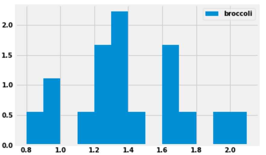
Using the code,
prices.plot(kind='hist', y='broccoli', bins=np.arange(0.8, 2.11, 0.1), density=True)we produced the histogram below:
How many grocery stores sold broccoli for a price greater than or equal to $1.30 per pound, but less than $1.40 per pound (the tallest bar)?
Answer: 4 grocery stores
We are given that the bins start at 0.8 and have a width of 0.1, which means one of the bins has endpoints 1.3 and 1.4. This bin (the tallest bar) includes all grocery stores that sold broccoli for a price greater than or equal to $1.30 per pound, but less than $1.40 per pound.
This bar has a width of 0.1 and we’d estimate the height to be around 2.2, though we can’t say exactly. Multiplying these values, the area of the bar is about 0.22, which means about 22 percent of the grocery stores fall into this bin. There are 18 grocery stores in total, as we are told in the introduction to this question. We can compute using a calculator that 22 percent of 18 is 3.96. Since the actual number of grocery stores this represents must be a whole number, this bin must represent 4 grocery stores.
The reason for the slight discrepancy between 3.96 and 4 is that we used 2.2 for the height of the bar, a number that we determined by eye. We don’t know the exact height of the bar. It is reassuring to do the calculation and get a value that’s very close to an integer, since we know the final answer must be an integer.
The average score on this problem was 71%.
Suppose we now plot the same data with different bins, using the following line of code:
prices.plot(kind='hist', y='broccoli', bins=[0.8, 1, 1.1, 1.5, 1.8, 1.9, 2.5], density=True)What would be the height on the y-axis for the bin corresponding to the interval [\$1.10, \$1.50)? Input your answer below.
Answer: 1.25
First, we need to figure out how many grocery stores the bin [\$1.10, \$1.50) contains. We already know from the previous subpart that there are four grocery stores in the bin [\$1.30, \$1.40). We could do similar calculations to find the number of grocery stores in each of these bins:
However, it’s much simpler and faster to use the fact that when the bins are all equally wide, the height of a bar is proportional to the number of data values it contains. So looking at the histogram in the previous subpart, since we know the [\$1.30, \$1.40) bin contains 4 grocery stores, then the [\$1.10, \$1.20) bin must contain 1 grocery store, since it’s only a quarter as tall. Again, we’re taking advantage of the fact that there must be an integer number of grocery stores in each bin when we say it’s 1/4 as tall. Our only options are 1/4, 1/2, or 3/4 as tall, and among those choices, it’s clear.
Therefore, by looking at the relative heights of the bars, we can quickly determine the number of grocery stores in each bin:
Adding these numbers together, this means there are 9 grocery stores whose broccoli prices fall in the interval [\$1.10, \$1.50). In the new histogram, these 9 grocery stores will be represented by a bar of width 1.50-1.10 = 0.4. The area of the bar should be \frac{9}{18} = 0.5. Therefore the height must be \frac{0.5}{0.4} = 1.25.
The average score on this problem was 33%.
You are interested in finding out the number of stores in which a pint of ice cream was cheaper than a pound of broccoli. Will you be able to determine the answer to this question by looking at the plot produced by the code below?
prices.get(['broccoli', 'ice_cream']).plot(kind='barh')Yes
No
Answer: Yes
When we use .plot without specifying a y
column, it uses every column in the DataFrame as a y column
and creates an overlaid plot. Since we first use get with
the list ['broccoli', 'ice_cream'], this keeps the
'broccoli' and 'ice_cream' columns from
prices, so our bar chart will overlay broccoli prices with
ice cream prices. Notice that this get is unnecessary
because prices only has these two columns, so it would have
been the same to just use prices directly. The resulting
bar chart will look something like this:
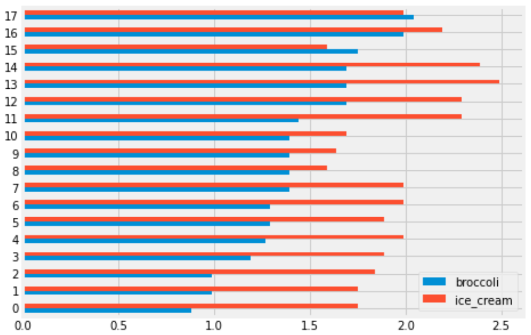
Each grocery store has its broccoli price represented by the length of the blue bar and its ice cream price represented by the length of the red bar. We can therefore answer the question by simply counting the number of red bars that are shorter than their corresponding blue bars.
The average score on this problem was 78%.
You are interested in finding out the number of stores in which a pint of ice cream was cheaper than a pound of broccoli. Will you be able to determine the answer to this question by looking at the plot produced by the code below?
prices.get(['broccoli', 'ice_cream']).plot(kind='hist')Yes
No
Answer: No
This will create an overlaid histogram of broccoli prices and ice cream prices. So we will be able to see the distribution of broccoli prices together with the distribution of ice cream prices, but we won’t be able to pair up particular broccoli prices with ice cream prices at the same store. This means we won’t be able to answer the question. The overlaid histogram would look something like this:
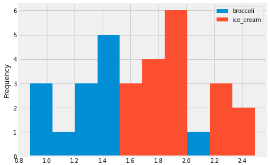
This tells us that broadly, ice cream tends to be more expensive than broccoli, but we can’t say anything about the number of stores where ice cream is cheaper than broccoli.
The average score on this problem was 81%.
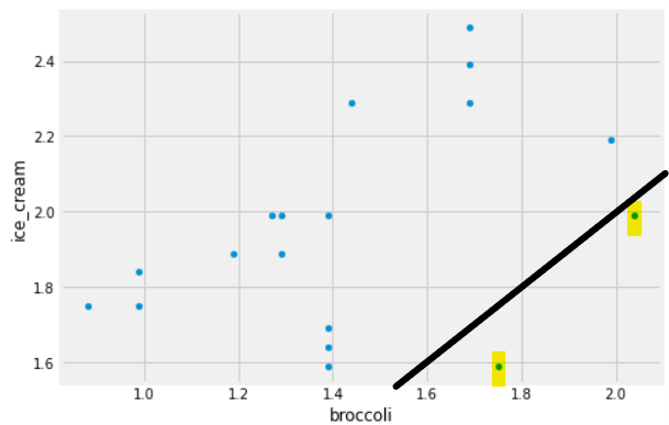
Some code and the scatterplot that produced it is shown below:
(prices.get(['broccoli', 'ice_cream']).plot(kind='scatter', x='broccoli', y='ice_cream'))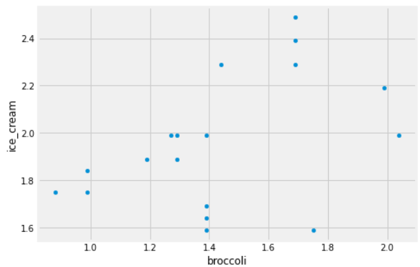
Can you use this plot to figure out the number of stores in which a pint of ice cream was cheaper than a pound of broccoli?
If so, say how many such stores there are and explain how you came to that conclusion.
If not, explain why this scatterplot cannot be used to answer the question.
Answer: Yes, and there are 2 such stores.
In this scatterplot, each grocery store is represented as one dot. The x-coordinate of that dot tells the price of broccoli at that store, and the y-coordinate tells the price of ice cream. If a grocery store’s ice cream price is cheaper than its broccoli price, the dot in the scatterplot will have y<x. To identify such dots in the scatterplot, imagine drawing the line y=x. Any dot below this line corresponds to a point with y<x, which is a grocery store where ice cream is cheaper than broccoli. As we can see, there are two such stores.
The average score on this problem was 78%.
Note: This problem is out of scope; it covers material no longer included in the course.
You have a DataFrame called flights containing
information on various plane tickets sold between US cities. The columns
are 'route_length', which stores distance between the
arrival and departure airports, in miles, and 'price',
which stores the cost of the airline ticket, in dollars. You notice that
longer flights tend to cost more, as expected.
| route_length | price |
|---|---|
| 2500 | 249 |
| 2750 | 249 |
| 2850 | 349 |
| 2850 | 319 |
| 2950 | 329 |
| 2950 | 309 |
| 3000 | 349 |
You want to use your data, shown in full above, to predict the
price of an airline ticket for a route that is 2800 miles long. What
would Galton’s method predict for the price of your ticket, if we
consider “nearby” to mean within 6o miles? Give your answer to the
nearest dollar.
Answer: 306 dollars
Galton’s method for making predictions is to take “nearby” x-values and average their corresponding y-values. For example, to predict the height of a child born to 70-inch parents, he averages the heights of children born to families where the parents are close to 70 inches tall. Using that same strategy here, we first need to identify which flights are considered “nearby” to a route that is 2800 miles. We are told that “nearby” means within 60 miles, so we are looking for flights between 2740 and 2860 miles in length. There are three such flights (the second, third, and fourth rows of the original data):
| route_length | price |
|---|---|
| 2750 | 249 |
| 2850 | 349 |
| 2850 | 319 |
Now, we simply need to average these three prices to make our
prediction. Since \frac{249+349+319}{3} =
305.67 and we are told to round to the nearest dollar, our
prediction is 306 dollars.
The average score on this problem was 59%.
You generate a three-digit number by randomly choosing each digit to be a number 0 through 9, inclusive. Each digit is equally likely to be chosen.
What is the probability you produce the number 027? Give your answer as a decimal number between 0 and 1 with no rounding.
Answer: 0.001
There is a \frac{1}{10} chance that we get 0 as the first random number, a \frac{1}{10} chance that we get 2 as the second random number, and a \frac{1}{10} chance that we get 7 as the third random number. The probability of all of these events happening is \frac{1}{10}*\frac{1}{10}*\frac{1}{10} = 0.001.
Another way to do this problem is to think about the possible outcomes. Any number from 000 to 999 is possible and all are equally likely. Since there are 1000 possible outcomes and the number 027 is just one of the possible outcomes, the probability of getting this outcome is \frac{1}{1000} = 0.001.
The average score on this problem was 92%.
What is the probability you produce a number with an odd digit in the middle position? For example, 250. Give your answer as a decimal number between 0 and 1 with no rounding.
Answer: 0.5
Because the values of the left and right positions are not important to us, think of the middle position only. When selecting a random number to go here, we are choosing randomly from the numbers 0 through 9. Since 5 of these numbers are odd (1, 3, 5, 7, 9), the probability of getting an odd number is \frac{5}{10} = 0.5.
The average score on this problem was 78%.
What is the probability you produce a number with a 7 in it somewhere? Give your answer as a decimal number between 0 and 1 with no rounding.
Answer: 0.271
It’s easier to calculate the probability that the number has no 7 in it, and then subtract this probability from 1. To solve this problem directly, we’d have to consider cases where 7 appeared multiple times, which would be more complicated.
The probability that the resulting number has no 7 is \frac{9}{10}*\frac{9}{10}*\frac{9}{10} = 0.729 because in each of the three positions, there is a \frac{9}{10} chance of selecting something other than a 7. Therefore, the probability that the number has a 7 is 1 - 0.729 = 0.271.
The average score on this problem was 69%.
Describe in your own words the difference between a probability distribution and an empirical distribution. Give an example of what each distribution might look like for a certain experiment. Choose an experiment that we have not already seen in this class.
Answer: There are many possible correct answers. Below are some student responses that earned full credit, lightly edited for clarity.
Probability distributions are theoretical distributions distributed over all possible values of an experiment. Meanwhile, empirical distributions are distributions of the real observed data. An example of this would be choosing a certain suit from a deck of cards. The probability distribution would be uniform, with a 1/4 chance of choosing each suit. Meanwhile, the empirical distribution of choosing suits from a deck of cards in 50 pulls manually and graphing the observed data would show us different chances.
A probability distribution is the distribution describing the theoretical probability of each potential value occurring in an experiment, while the empirical distribution describes the proportion of each of the values in the experiment after running it, including all observed values. In other words, the probability distribution is what we expect to happen, and the empirical distribution is what actually happens.
For example: My friends and I often go to a food court to eat, and we randomly pick a restaurant every time. There is 1 McDonald’s, 1 Subway, and 2 Panda Express restaurants in the food court.
The probability distribution is as follows:
After going to the food court 100 times, we look at the empirical distribution to see which restaurants we eat at most often. it is as follows:
Probability distribution is a theoretical representation of certain outcomes in an event whereas an empirical distribution is the observational representation of the same outcomes in an event produced from an experiment.
An example would be if I had 10 pairs of shoes in my closet: The probability distribution would suggest that each pair of shoes has an equal chance of getting picked on any given day. On the other hand, an empirical distribution would be drawn by recording which pair got picked on a given day in N trials.
The average score on this problem was 82%.
results = np.array([])
for i in np.arange(10):
    result = np.random.choice(np.arange(1000), replace=False)
    results = np.append(results, result)
After this code executes, results contains:
a simple random sample of size 9, chosen from a set of size 999 with replacement
a simple random sample of size 9, chosen from a set of size 999 without replacement
a simple random sample of size 10, chosen from a set of size 1000 with replacement
a simple random sample of size 10, chosen from a set of size 1000 without replacement
Answer: a simple random sample of size 10, chosen from a set of size 1000 with replacement
Let’s see what the code is doing. The first line initializes an empty
array called results. The for loop runs 10 times. Each
time, it creates a value called result by some process
we’ll inspect shortly and appends this value to the end of the
results array. At the end of the code snippet,
results will be an array containing 10 elements.
Now, let’s look at the process by which each element
result is generated. Each result is a random
element chosen from np.arange(1000) which is the numbers
from 0 to 999, inclusive. That’s 1000 possible numbers. Each time
np.random.choice is called, just one value is chosen from
this set of 1000 possible numbers.
When we sample just one element from a set of values, sampling with replacement is the same as sampling without replacement, because sampling with or without replacement concerns whether subsequent draws can be the same as previous ones. When we’re just sampling one element, it really doesn’t matter whether our process involves putting that element back, as we’re not going to draw again!
Therefore, result is just one random number chosen from
the 1000 possible numbers. Each time the for loop executes,
result gets set to a random number chosen from the 1000
possible numbers. It is possible (though unlikely) that the random
result of the first execution of the loop matches the
result of the second execution of the loop. More generally,
there can be repeated values in the results array since
each entry of this array is independently drawn from the same set of
possibilities. Since repetitions are possible, this means the sample is
drawn with replacement.
Therefore, the results array contains a sample of size
10 chosen from a set of size 1000 with replacement. This is called a
“simple random sample” because each possible sample of 10 values is
equally likely, which comes from the fact that
np.random.choice chooses each possible value with equal
probability by default.
The average score on this problem was 11%.
Suppose we take a uniform random sample with replacement from a population, and use the sample mean as an estimate for the population mean. Which of the following is correct?
If we take a larger sample, our sample mean will be closer to the population mean.
If we take a smaller sample, our sample mean will be closer to the population mean.
If we take a larger sample, our sample mean is more likely to be close to the population mean than if we take a smaller sample.
If we take a smaller sample, our sample mean is more likely to be close to the population mean than if we take a larger sample.
Answer: If we take a larger sample, our sample mean is more likely to be close to the population mean than if we take a smaller sample.
Larger samples tend to give better estimates of the population mean than smaller samples. That’s because large samples are more like the population than small samples. We can see this in the extreme. Imagine a sample of 1 element from a population. The sample might vary a lot, depending on the distribution of the population. On the other extreme, if we sample the whole population, our sample mean will be exactly the same as the population mean.
Notice that the correct answer choice uses the words “is more likely to be close to” as opposed to “will be closer to.” We’re talking about a general phenomenon here: larger samples tend to give better estimates of the population mean than smaller samples. We cannot say that if we take a larger sample our sample mean “will be closer to” the population mean, since it’s always possible to get lucky with a small sample and unlucky with a large sample. That is, one particular small sample may happen to have a mean very close to the population mean, and one particular large sample may happen to have a mean that’s not so close to the population mean. This can happen, it’s just not likely to.
The average score on this problem was 100%.