
← return to practice.dsc10.com
Instructor(s): Suraj Rampure
This exam was administered remotely via Gradescope. The exam was open-internet, and students were able to use Jupyter Notebooks. They had 3 hours to work on it.
Note (groupby / pandas 2.0): Pandas 2.0+ no longer
silently drops columns that can’t be aggregated after a
groupby, so code written for older pandas may behave
differently or raise errors. In these practice materials we use
.get() to select the column(s) we want after
.groupby(...).mean() (or other aggregations) so that our
solutions run on current pandas. On real exams you will not be penalized
for omitting .get() when the old behavior would have
produced the same answer.
Welcome to the Final Exam for DSC 10 Winter 2022! In this exam, we will use data from the 2021 Women’s National Basketball Association (WNBA) season. In basketball, players score points by shooting the ball into a hoop. The team that scores the most points wins the game.
Kelsey Plum, a WNBA player, attended La Jolla Country Day School,
which is adjacent to UCSD’s campus. Her current team is the Las Vegas
Aces (three-letter code 'LVA'). In 2021, the Las
Vegas Aces played 31 games, and Kelsey Plum played in all
31.
The DataFrame plum contains her stats for all games the
Las Vegas Aces played in 2021. The first few rows of plum
are shown below (though the full DataFrame has 31 rows, not 5):
Each row in plum corresponds to a single game. For each
game, we have:
'Date' (str), the date on which the game
was played'Opp' (str), the three-letter code of the
opponent team'Home' (bool), True if the
game was played in Las Vegas (“home”) and False if it was
played at the opponent’s arena (“away”)'Won' (bool), True if the Las
Vegas Aces won the game and False if they lost'PTS' (int), the number of points Kelsey
Plum scored in the game'AST' (int), the number of assists
(passes) Kelsey Plum made in the game'TOV' (int), the number of turnovers
Kelsey Plum made in the game (a turnover is when you lose the ball –
turnovers are bad!)Tip: Open this page in another tab, so that it is easy to refer to this data description as you work through the exam.
What type of visualization is best suited for visualizing the trend in the number of points Kelsey Plum scored per game in 2021?
Histogram
Bar chart
Line chart
Scatter plot
Answer: Line chart
Here, there are two quantitative variables (number of points and game number), and one of them involves some element of time (game number). Line charts are appropriate when one quantitative variable is time.
The average score on this problem was 75%.
Fill in the blanks below so that total_june evaluates to
the total number of points Kelsey Plum scored in June.
june_only = plum[__(a)__]
total_june = june_only.__(b)__
What goes in blank (a)?
What goes in blank (b)?
Answer:
plum.get('Date').str.contains('-06-')
get('PTS').sum()
To find the total number of points Kelsey Plum scored in June, one
approach is to first create a DataFrame with only the rows for June.
During the month of June, the 'Date' values contain
'-06-' (since June is the 6th month), so
plum.get('Date').str.contains('-06-') is a Series
containing True only for the June rows and
june_only = plum[plum.get('Date').str.contains('-06-')] is
a DataFrame containing only the June rows.
Then, all we need is the sum of the 'PTS' column, which
is given by june_only.get('PTS').sum().
The average score on this problem was 90%.
Consider the function unknown, defined below.
def unknown(df):
    grouped = plum.groupby('Opp').max().get(['Date', 'PTS'])
    return np.array(grouped.reset_index().index)[df]
What does unknown(3) evaluate to?
'2021-06-05'
'WAS'
The date on which Kelsey Plum scored the most points
The three-letter code of the opponent on which Kelsey Plum scored the most points
The number 0
The number 3
An error
Answer: The number 3
plum.groupby('Opp').max() finds the largest value in the
'Date', 'Home', 'Won',
'PTS', 'AST', and 'TOV' columns
for each unique 'Opp' (independently for each column).
grouped = plum.groupby('Opp').max().get(['Date', 'PTS'])
keeps only the 'Date' and 'PTS' columns. Note
that in grouped, the index is 'Opp', the
column we grouped on.
When grouped.reset_index() is called, the index is
switched back to the default of 0, 1, 2, 3, 4, and so on. Then,
grouped.reset_index().index is an Index
containing the numbers [0, 1, 2, 3, 4, ...], and
np.array(grouped.reset_index().index) is
np.array([0, 1, 2, 3, 4, ...]). In this array, the number
at position i is just i, so the number at
position df is df. Here, df is
the argument to unknown, and we were asked for the value of
unknown(3), so the correct answer is the number at position
3 in np.array([0, 1, 2, 3, 4, ...]) which is 3.
Note that if we asked for unknown(50) (or
unknown(k), where k is any integer above 30),
the answer would be “An error”, since grouped could not
have had 51 rows. plum has 31 rows, so grouped
has at most 31 rows (but likely less, since Kelsey Plum’s team likely
played the same opponent multiple times).
The average score on this problem was 72%.
For your convenience, we show the first few rows of plum
again below.
Suppose that Plum’s team, the Las Vegas Aces, won at least one game in Las Vegas and lost at least one game in Las Vegas. Also, suppose they won at least one game in an opponent’s arena and lost at least one game in an opponent’s arena.
Consider the DataFrame home_won, defined below.
home_won = plum.groupby(['Home', 'Won']).mean().reset_index()How many rows does home_won have?
How many columns does home_won have?
Answer: 4 rows and 5 columns.
plum.groupby(['Home', 'Won']).mean() contains one row
for every unique combination of 'Home' and
'Won'. There are two values of 'Home' -
True and False – and two values of
'Won' – True and False – leading
to 4 combinations. We can assume that there was at least one row in
plum for each of these 4 combinations due to the assumption
given in the problem:
Suppose that Plum’s team, the Las Vegas Aces, won at least one game in Las Vegas and lost at least one game in Las Vegas. Also, suppose they won at least one game in an opponent’s arena and lost at least one game in an opponent’s arena.
plum started with 7 columns: 'Date',
'Opp', 'Home', 'Won',
'PTS', 'AST', and 'TOV'. After
grouping by ['Home', 'Won'] and using .mean(),
'Home' and 'Won' become the index. The
resulting DataFrame contains all of the columns that the
.mean() aggregation method can work on. We cannot take the
mean of 'Date' and 'Opp', because those
columns are strings, so
plum.groupby(['Home', 'Won']).mean() contains a
MultiIndex with 2 “columns” – 'Home' and
'Won' – and 3 regular columns – 'PTS'
'AST', and 'TOV'. Then, when using
.reset_index(), 'Home' and 'Won'
are restored as regular columns, meaning that
plum.groupby(['Home', 'Won']).mean().reset_index() has
2 + 3 = 5 columns.
The average score on this problem was 78%.
Consider the DataFrame home_won once again.
home_won = plum.groupby(['Home', 'Won']).mean().reset_index()Now consider the DataFrame puzzle, defined below. Note
that the only difference between home_won and
puzzle is the use of .count() instead of
.mean().
puzzle = plum.groupby(['Home', 'Won']).count().reset_index()How do the number of rows and columns in home_won
compare to the number of rows and columns in puzzle?
home_won and puzzle have the same number of
rows and columns
home_won and puzzle have the same number of
rows, but a different number of columns
home_won and puzzle have the same number of
columns, but a different number of rows
home_won and puzzle have both a different
number of rows and a different number of columns
Answer: home_won and
puzzle have the same number of rows, but a different number
of columns
All that changed between home_won and
puzzle is the aggregation method. The aggregation method
has no influence on the number of rows in the output DataFrame, as there
is still one row for each of the 4 unique combinations of
'Home' and 'Won'.
However, puzzle has 7 columns, instead of 5. In the
solution to the above subpart, we noticed that we could not use
.mean() on the 'Date' and 'Opp'
columns, since they contained strings. However, we can use
.count() (since .count() just determines the
number of non-NA values in each group), and so the 'Date'
and 'Opp' columns are not “lost” when aggregating. Hence,
puzzle has 2 more columns than home_won.
The average score on this problem was 85%.
For your convenience, we show the first few rows of plum
again below.
There is exactly one team in the WNBA that Plum’s team did not win
any games against during the 2021 season. Fill in the blanks below so
that never_beat evaluates to a string containing the
three-letter code of that team.
never_beat = plum.groupby(__(a)__).sum().__(b)__What goes in blank (a)?
What goes in blank (b)?
Answer:
'Opp'
sort_values('Won').index[0]
The key insight here is that the values in the 'Won'
column are Boolean, and when Boolean values are used in arithmetic they
are treated as 1s (True) and 0s (False). The
sum of several 'Won' values is the same as the
number of wins.
If we group plum by 'Opp' and use
.sum(), the resulting 'Won' column contains
the number of wins that Plum’s team had against each unique opponent. If
we sort this DataFrame by 'Won' in increasing order (which
is the default behavior of sort_values), the row at the top
will correspond to the 'Opp' that Plum’s team had no wins
against. Since we grouped by 'Opp', team names are stored
in the index, so .index[0] will give us the name of the
desired team.
The average score on this problem was 67%.
Recall that plum has 31 rows, one corresponding to each
of the 31 games Kelsey Plum’s team played in the 2021 WNBA season.
Fill in the blank below so that win_bool evaluates to
True.
def modify_series(s):
    return __(a)__

n_wins = plum.get('Won').sum()
win_bool = n_wins == (31 + modify_series(plum.get('Won')))
What goes in blank (a)?
-s.sum()
-(s == False).sum()
len(s) - s.sum()
not s.sum()
-s[s.get('Won') == False].sum()
Answer: -(s == False).sum()
n_wins equals the number of wins that Plum’s team had.
Recall that her team played 31 games in total. In order for
(31 + modify_series(plum.get('Won'))) to be equal to her
team’s number of wins, modify_series(plum.get('Won')) must
be equal to her team’s number of losses, multiplied by -1.
To see this algebraically, let
modified = modify_series(plum.get('Won')). Then:
31 + \text{modified} = \text{wins} \text{modified} = \text{wins} - 31 = -(31 - \text{wins}) = -(\text{losses})
The function modified_series(s) takes in a Series
containing the wins and losses for each of Plum’s team’s games and needs
to return the number of losses multiplied by -1. s.sum()
returns the number of wins, and (s == False).sum() returns
the number of losses. Then, -(s == False).sum() returns the
number of losses multiplied by -1, as desired.
The average score on this problem was 76%.
Let’s suppose there are 4 different types of shots a basketball player can take – layups, midrange shots, threes, and free throws.
The DataFrame breakdown has 4 rows and 50 columns – one
row for each of the 4 shot types mentioned above, and one column for
each of 50 different players. Each column of breakdown
describes the distribution of shot types for a single player.
The first few columns of breakdown are shown below.
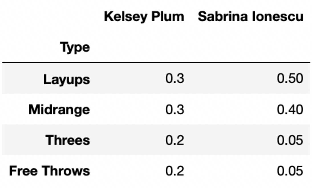
For instance, 30% of Kelsey Plum’s shots are layups, 30% of her shots are midrange shots, 20% of her shots are threes, and 20% of her shots are free throws.
Below, we’ve drawn an overlaid bar chart showing the shot distributions of Kelsey Plum and Chiney Ogwumike, a player on the Los Angeles Sparks.
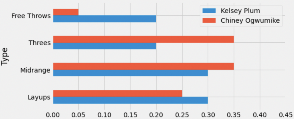
What is the total variation distance (TVD) between Kelsey Plum’s shot distribution and Chiney Ogwumike’s shot distribution? Give your answer as a proportion between 0 and 1 (not a percentage) rounded to three decimal places.
Answer: 0.2
Recall, the TVD is the sum of the absolute differences in proportions, divided by 2. The absolute differences in proportions for each category are as follows:
Then, we have
\text{TVD} = \frac{1}{2} (0.15 + 0.15 + 0.05 + 0.05) = 0.2
The average score on this problem was 84%.
Recall, breakdown has information for 50 different
players. We want to find the player whose shot distribution is the
most similar to Kelsey Plum, i.e. has the lowest TVD
with Kelsey Plum’s shot distribution.
Fill in the blanks below so that most_sim_player
evaluates to the name of the player with the most similar shot
distribution to Kelsey Plum. Assume that the column named
'Kelsey Plum' is the first column in breakdown
(and again that breakdown has 50 columns total).
most_sim_player = ''
lowest_tvd_so_far = __(a)__
other_players = np.array(breakdown.columns).take(__(b)__)
for player in other_players:
    player_tvd = tvd(breakdown.get('Kelsey Plum'),
                     breakdown.get(player))
    if player_tvd < lowest_tvd_so_far:
        lowest_tvd_so_far = player_tvd
__(c)__-1
-0.5
0
0.5
1
np.array([])
''
What goes in blank (b)?
What goes in blank (c)?
Answers: 1, np.arange(1, 50),
most_sim_player = player
Let’s try and understand the code provided to us. It appears that
we’re looping over the names of all other players, each time computing
the TVD between Kelsey Plum’s shot distribution and that player’s shot
distribution. If the TVD calculated in an iteration of the
for-loop (player_tvd) is less than the
previous lowest TVD (lowest_tvd_so_far), the current player
(player) is now the most “similar” to Kelsey Plum, and so
we store their TVD and name (in most_sim_player).
Before the for-loop, we haven’t looked at any other
players, so we don’t have values to store in
most_sim_player and lowest_tvd_so_far. On the
first iteration of the for-loop, both of these values need
to be updated to reflect Kelsey Plum’s similarity with the first player
in other_players. This is because, if we’ve only looked at
one player, that player is the most similar to Kelsey Plum.
most_sim_player is already initialized as an empty string,
and we will specify how to “update” most_sim_player in
blank (c). For blank (a), we need to pick a value of
lowest_tvd_so_far that we can guarantee
will be updated on the first iteration of the for-loop.
Recall, TVDs range from 0 to 1, with 0 meaning “most similar” and 1
meaning “most different”. This means that no matter what, the TVD
between Kelsey Plum’s distribution and the first player’s distribution
will be less than 1*, and so if we initialize
lowest_tvd_so_far to 1 before the for-loop, we
know it will be updated on the first iteration.
lowest_tvd_so_far and
most_sim_player wouldn’t be updated on the first iteration.
Rather, they’d be updated on the first iteration where
player_tvd is strictly less than 1. (We’d expect that the
TVDs between all pairs of players are neither exactly 0 nor exactly 1,
so this is not a practical issue.) To avoid this issue entirely, we
could change if player_tvd < lowest_tvd_so_far to
if player_tvd <= lowest_tvd_so_far, which would make
sure that even if the first TVD is 1, both
lowest_tvd_so_far and most_sim_player are
updated on the first iteration.lowest_tvd_so_far
to a value larger than 1 as well. Suppose we initialized it to 55 (an
arbitrary positive integer). On the first iteration of the
for-loop, player_tvd will be less than 55, and
so lowest_tvd_so_far will be updated.Then, we need other_players to be an array containing
the names of all players other than Kelsey Plum, whose name is stored at
position 0 in breakdown.columns. We are told that there are
50 players total, i.e. that there are 50 columns in
breakdown. We want to take the elements in
breakdown.columns at positions 1, 2, 3, …, 49 (the last
element), and the call to np.arange that generates this
sequence of positions is np.arange(1, 50). (Remember,
np.arange(a, b) does not include the second integer!)
In blank (c), as mentioned in the explanation for blank (a), we need
to update the value of most_sim_player. (Note that we only
arrive at this line if player_tvd is the lowest pairwise
TVD we’ve seen so far.) All this requires is
most_sim_player = player, since player
contains the name of the player who we are looking at in the current
iteration of the for-loop.
The average score on this problem was 70%.
Let’s again consider the shot distributions of Kelsey Plum and Cheney Ogwumike.
We define the maximum squared distance (MSD) between two categorical distributions as the largest squared difference between the proportions of any category.
What is the MSD between Kelsey Plum’s shot distribution and Chiney Ogwumike’s shot distribution? Give your answer as a proportion between 0 and 1 (not a percentage) rounded to three decimal places.
Answer: 0.023
Recall, in the solution to the first subpart of this problem, we calculated the absolute differences between the proportions of each category.
The squared differences between the proportions of each category are computed by squaring the results in the list above (e.g. for Free Throws we’d have (0.05 - 0.2)^2 = 0.15^2). To find the maximum squared difference, then, all we need to do is find the largest of 0.15^2, 0.15^2, 0.05^2, and 0.05^2. Since 0.15 > 0.05, we have that the maximum squared distance is 0.15^2 = 0.0225, which rounds to 0.023.
The average score on this problem was 85%.
For your convenience, we show the first few columns of
breakdown again below.
In basketball:
Suppose that Kelsey Plum is guaranteed to shoot exactly 10 shots a
game. The type of each shot is drawn from the 'Kelsey Plum'
column of breakdown (meaning that, for example, there is a
30% chance each shot is a layup).
Fill in the blanks below to complete the definition of the function
simulate_points, which simulates the number of points
Kelsey Plum scores in a single game. (simulate_points
should return a single number.)
def simulate_points():
    shots = np.random.multinomial(__(a)__, breakdown.get('Kelsey Plum'))
    possible_points = np.array([2, 2, 3, 1])
return __(b)__Answers: 10,
(shots * possible_points).sum()
To simulate the number of points Kelsey Plum scores in a single game, we need to:
To simulate the number of shots she takes of each type, we use
np.random.multinomial. This is because each shot,
independently of all other shots, has a 30% chance of being a layup, a
30% chance of being a midrange, and so on. What goes in blank (a) is the
number of shots she is taking in total; here, that is 10.
shots will be an array of length 4 containing the number of
shots of each type - for instance, shots may be
np.array([3, 4, 2, 1]), which would mean she took 3 layups,
4 midranges, 2 threes, and 1 free throw.
Now that we have shots, we need to factor in how many
points each type of shot is worth. This can be accomplished by
multiplying shots with possible_points, which
was already defined for us. Using the example where shots
is np.array([3, 4, 2, 1]),
shots * possible_points evaluates to
np.array([6, 8, 6, 1]), which would mean she scored 6
points from layups, 8 points from midranges, and so on. Then, to find
the total number of points she scored, we need to compute the sum of
this array, either using the np.sum function or
.sum() method. As such, the two correct answers for blank
(b) are (shots * possible_points).sum() and
np.sum(shots * possible_points).
The average score on this problem was 84%.
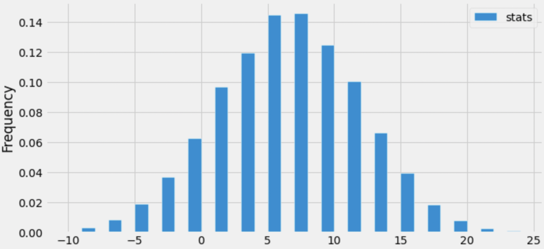
True or False: If we call simulate_points() 10,000 times
and plot a histogram of the results, the distribution will look roughly
normal.
True
False
Answer: True
The answer is True because of the Central Limit Theorem. Recall, the
CLT states that no matter what the population distribution looks like,
if you take many repeated samples with replacement, the distribution of
the sample means and sample sums will be roughly normal.
simulate_points() returns the sum of a sample of size 10
drawn with replacement from a population, and so if we generate many
sample sums, the distribution of those sample sums will be roughly
normal.
The distribution we are drawing from is the one below.
| Type | Points | Probability |
|---|---|---|
| Layups | 2 | 0.3 |
| Midrange | 2 | 0.3 |
| Threes | 3 | 0.2 |
| Free Throws | 1 | 0.2 |
The average score on this problem was 78%.
ESPN (a large sports news network) states that the Las Vegas Aces have a 60% chance of winning their upcoming game. You’re curious as to how they came up with this estimate, and you decide to conduct a hypothesis test for the following hypotheses:
Null Hypothesis: The Las Vegas Aces win each game with a probability of 60%.
Alternative Hypothesis: The Las Vegas Aces win each game with a probability above 60%.
In both hypotheses, we are assuming that each game is independent of all other games.
In the 2021 season, the Las Vegas Aces won 22 of their games and lost 9 of their games.
Below, we have provided the code necessary to conduct the hypothesis test described above.
stats = np.array([])
for i in np.arange(10000):
    sim = np.random.multinomial(31, [0.6, 0.4])
    stat = fn(sim)
    stats = np.append(stats, stat)
win_p_value = np.count_nonzero(stats >= fn([22, 9])) / 10000
fn is a function that computes a test
statistic, given a list or array arr of two elements (the
first of which is the number of wins, and the second of which is the
number of losses). You can assume that neither element of
arr is equal to 0.
Below, we define 5 possible test statistics fn.
Option 1:
def fn(arr):
    return arr[0] / arr[1]
Option 2:
def fn(arr):
    return arr[0]
Option 3:
def fn(arr):
    return np.abs(arr[0] - arr[1])
Option 4:
def fn(arr):
    return arr[0] - arr[1]
Option 5:
def fn(arr):
    return arr[1] - arr[0]
Which of the above functions fn would be valid test
statistics for this hypothesis test and p-value calculation?
Select all that apply.
Option 1
Option 2
Option 3
Option 4
Option 5
Answer: Options 1, 2, and 4
In the code provided to us, stats is an array containing
10,000 p-values generated by the function fn (note that we
are appending stat to stats, and in the line
before that we have stat = fn(sim)). In the very last line
of the code provided, we have:
win_p_value = np.count_nonzero(stats >= fn([22, 9])) / 10000If we look closely, we see that we are computing the p-value by
computing the proportion of simulated test statistics that were
greater than or equal to (>=) the observed
statistic. Since a p-value is computed as the proportion of
simulated test statistics that were as or more extreme than the
observed statistic, here it must mean that “big” test
statistics are more extreme.
Remember, the direction that is “extreme” is determined by our
alternative hypothesis. Here, the alternative hypothesis is that the Las
Vegas Aces win each game with a probability above 60%. As such, the test
statistic(s) we choose must be large when the probability that
the Aces win a game is high, and small when the probability
that the Aces win a game is low. With this all in mind, we can take a
look at the 5 options, remembering that arr[0] is
the number of simulated wins and arr[1] is the number of
simulated losses in a season of 31 games. This means that when
the Aces win more than they lose, arr[0] > arr[1], and
when they lose more than they win, arr[0] < arr[1].
arr[0] / arr[1]. If the Aces win a
lot, the numerator will be larger than the denominator, so this ratio
will be large. If the Aces lose a lot, the numerator will be smaller
than the denominator, and so this ratio will be small. This is what we
want!arr[0]. If the Aces win a lot, this number will
be large, and if the Aces lose a lot, this number will be small. This is
what we want!np.abs(arr[0] - arr[1]). If the Aces win a lot, then
arr[0] - arr[1] will be large, and so will
np.abs(arr[0] - arr[1]). This seems fine.
However, if the Aces lose a lot, then
arr[0] - arr[1] will be small (negative), but
np.abs(arr[0] - arr[1]) will still be large and positive.
This test statistic doesn’t allow us to differentiate
when the Aces win a lot or lose a lot, so we can’t use it as a test
statistic for our alternative hypothesis.arr[0] - arr[1] is large.
Furthermore, when the Aces lose a lot, arr[0] - arr[1] is
small (negative numbers are small in this context). This works!arr[1] - arr[0] is the
opposite of arr[0] - arr[1] in Option 4. When the Aces win
a lot, arr[1] - arr[0] is small (negative), and when the
Aces lose a lot, arr[1] - arr[0] is large (positive). This
is the opposite of what we want, so Option 5 does not work.
The average score on this problem was 77%.
The empirical distribution of one of the 5 test statistics presented
in the previous subpart is shown below. To draw the histogram, we used
the argument bins=np.arange(-10, 25).
Which test statistic does the above empirical distribution belong to?
Option 1
Option 2
Option 3
Option 4
Option 5
Answer: Option 4
The distribution visualized in the histogram has the following unique values: -9, -7, -5, -3, …, 17, 19, 21, 23. Crucially, the test statistic whose distribution we’ve visualized can both be positive and negative. Right off the bat, we can eliminate Options 1, 2, and 3:
arr[0]) by the number of losses
(arr[1]), and that quotient will always be a non-negative
number.arr[0]) will always be a non-negative number.np.abs(arr[0] - arr[1]), in this case) will
always be a non-negative number.Now, we must decide between Option 4, whose test statistic is “wins
minus losses” (arr[0] - arr[1]), and Option 5, whose test
statistic is “losses minus wins” (arr[1] - arr[0]).
First, let’s recap how we’re simulating. In the code
provided in the previous subpart, we have the line
sim = np.random.multinomial(31, [0.6, 0.4]). Each time we
run this line, sim will be set to an array with two
elements, the first of which we interpret as the number of simulated
wins and the second of which we interpret as the number of simulated
losses in a 31 game season. The first number in sim will
usually be larger than the second number in sim, since the
chance of a win (0.6) is larger than the chance of a loss (0.4). As
such, When we compute fn(sim) in the following line, the
difference between the wins and losses should typically be positive.
Back to our distribution. Note that the distribution provided in this subpart is centered at a positive number, around 7. Since the difference between wins and losses will typically be positive, it appears that we’ve visualized the distribution of the difference between wins and losses (Option 4). If we instead visualized the difference between losses and wins, the distribution should be centered at a negative number, but that’s not the case.
As such, the correct answer is Option 4.
The average score on this problem was 86%.
Consider the function fn_plus defined below.
def fn_plus(arr):
    return fn(arr) + 31
True or False: If fn is a valid test
statistic for the hypothesis test and p-value calculation presented at
the start of the problem, then fn_plus is also a valid test
statistic for the hypothesis test and p-value calculation presented at
the start of the problem.
True
False
Answer: True
All fn_plus is doing is adding 31 to the output of
fn. If we think in terms of pictures, the shape of
the distribution of fn_plus looks the same as the
distribution of fn, just moved to the right by 31 units.
Since the distribution’s shape is no different, the proportion of
simulated test statistics that are greater than the observed test
statistic is no different either, and so the p-value we calculate with
fn_plus is the same as the one we calculate with
fn.
The average score on this problem was 73%.
Below, we present the same code that is given at the start of the problem. (Remember to keep the data description from the top of the exam open in another tab!)
stats = np.array([])
for i in np.arange(10000):
    sim = np.random.multinomial(31, [0.6, 0.4])
    stat = fn(sim)
    stats = np.append(stats, stat)

win_p_value = np.count_nonzero(stats >= fn([22, 9])) / 10000
Below are four possible replacements for the line
sim = np.random.multinomial(31, [0.6, 0.4]).
Option 1:
def with_rep():
    won = plum.get('Won')
    return np.count_nonzero(np.random.choice(won, 31, replace=True))

sim = [with_rep(), 31 - with_rep()]
Option 2:
def with_rep():
    won = plum.get('Won')
    return np.count_nonzero(np.random.choice(won, 31, replace=True))

w = with_rep()
sim = [w, 31 - w]
Option 3:
def without_rep():
    won = plum.get('Won')
    return np.count_nonzero(np.random.choice(won, 31, replace=False))

sim = [without_rep(), 31 - without_rep()]
Option 4:
def perm():
    won = plum.get('Won')
    return np.count_nonzero(np.random.permutation(won))

w = perm()
sim = [w, 31 - w]
Which of the above four options could we replace the line
sim = np.random.multinomial(plum.shape[0], [0.6, 0.4]) with
and still perform a valid hypothesis test for the hypotheses stated at
the start of the problem?
Option 1
Option 2
Option 3
Option 4
Answer: Option 2
The line
sim = np.random.multinomial(plum.shape[0], [0.6, 0.4])
assigns sim to an array containing two numbers such
that:
We need to select an option that also creates such an array (or list,
in this case). Note that won = plum.get('Won'), a line that
is common to all four options, assigns won to a Series with
31 elements, each of which is either True or
False (corresponding to the wins and losses that the Las
Vegas Aces earned in their season).
Let’s take a look at the line
np.count_nonzero(np.random.choice(won, 31, replace=True)),
common to the first two options. Here, we are randomly selecting 31
elements from the Series won, with replacement, and
counting the number of Trues (since with
np.count_nonzero, False is counted as
0). Since we are making our selections with replacement,
each selected element has a \frac{22}{31} chance of being
True and a \frac{9}{31}
chance of being False (since won has 22
Trues and 9 Falses). As such,
np.count_nonzero(np.random.choice(won, 31, replace=True))
can be any integer between 0 and 31, inclusive.
Note that if we select without replacement
(replace=False) as Option 3 would like us to, then all 31
selected elements would be the same as the 31 elements in
won. As a result,
np.random.choice(won, 31, replace=False) will always have
22 Trues, just like won, and
np.count_nonzero(np.random.choice(won, 31, replace=True))
will always return 22. That’s not random, and so that’s not quite what
we’re looking for.
With this all in mind, let’s look at the four options.
with_rep(), we get a random number between 0 and 31
(inclusive), corresponding to the (random) number of simulated wins.
Then, we are assigning sim to be
[with_rep(), 31 - with_rep()]. However, it’s not guaranteed
that the two calls to with_rep return the same number of
wins, so it’s not guaranteed that sum(sim) is 31. Option 1,
then, is invalid.replace=False, and so without_rep() is always
22 and sim is always [22, 9]. The outcome is
not random.perm() always returns
the same number, 22. This is because all we are doing is shuffling the
entries in the won Series, but we aren’t changing the
number of wins (Trues) and losses (Falses). As
a result, w is always 22 and sim is always
[22, 9], making this non-random, just like in Option
3.By the process of elimination, Option 2 must be the
correct choice. It is similar to Option 1, but it only calls
with_rep once and “saves” the result to the name
w. As a result, w is random, and
w and 31 - w are guaranteed to sum to 31.
⚠️ Note: It turns out that none of these options run a valid hypothesis test, since the null hypothesis was that the Las Vegas Aces win 60% of their games but none of these simulation strategies use 60% anywhere (instead, they use the observation that the Aces actually won 22 games). However, this subpart was about the sampling strategies themselves, so this mistake from our end doesn’t invalidate the problem.
The average score on this problem was 70%.
Consider again the four options presented in the previous subpart.
In which of the four options is it guaranteed that
sum(sim) evaluates to 31? Select all that
apply.
Option 1
Option 2
Option 3
Option 4
Answers: Options 2, 3, and 4
with_rep evaluate to
different numbers (entirely possible, since it is random), then
sum(sim) will not be 31.sim is defined in
terms of some w. Specifically, w is some
number between 0 and 31 and sim is
[w, 31 - w], so sum(sim) is the same as
w + 31 - w, which is always 31.sim is always
[22, 9], and sum(sim) is always 31.
The average score on this problem was 72%.
Consider the definition of the function
diff_in_group_means:
def diff_in_group_means(df, group_col, num_col):
    s = df.groupby(group_col).mean().get(num_col)
return s.loc[False] - s.loc[True]It turns out that Kelsey Plum averages 0.61 more assists in games
that she wins (“winning games”) than in games that she loses (“losing
games”). Fill in the blanks below so that observed_diff
evaluates to -0.61.
observed_diff = diff_in_group_means(plum, __(a)__, __(b)__)What goes in blank (a)?
What goes in blank (b)?
Answers: 'Won', 'AST'
To compute the number of assists Kelsey Plum averages in winning and
losing games, we need to group by 'Won'. Once doing so, and
using the .mean() aggregation method, we need to access
elements in the 'AST' column.
The second argument to diff_in_group_means,
group_col, is the column we’re grouping by, and so blank
(a) must be filled by 'Won'. Then, the second argument,
num_col, must be 'AST'.
Note that after extracting the Series containing the average number
of assists in wins and losses, we are returning the value with the index
False (“loss”) minus the value with the index
True (“win”). So, throughout this problem, keep in mind
that we are computing “losses minus wins”. Since our observation was
that she averaged 0.61 more assists in wins than in losses, it makes
sense that diff_in_group_means(plum, 'Won', 'AST') is -0.61
(rather than +0.61).
The average score on this problem was 94%.
After observing that Kelsey Plum averages more assists in winning games than in losing games, we become interested in conducting a permutation test for the following hypotheses:
To conduct our permutation test, we place the following code in a
for-loop.
won = plum.get('Won')
ast = plum.get('AST')
shuffled = plum.assign(Won_shuffled=np.random.permutation(won)) \
               .assign(AST_shuffled=np.random.permutation(ast))
Which of the following options does not compute a valid simulated test statistic for this permutation test?
diff_in_group_means(shuffled, 'Won', 'AST')
diff_in_group_means(shuffled, 'Won', 'AST_shuffled')
diff_in_group_means(shuffled, 'Won_shuffled, 'AST')
diff_in_group_means(shuffled, 'Won_shuffled, 'AST_shuffled')
More than one of these options do not compute a valid simulated test statistic for this permutation test
Answer:
diff_in_group_means(shuffled, 'Won', 'AST')
As we saw in the previous subpart,
diff_in_group_means(shuffled, 'Won', 'AST') computes the
observed test statistic, which is -0.61. There is no randomness involved
in the observed test statistic; each time we run the line
diff_in_group_means(shuffled, 'Won', 'AST') we will see the
same result, so this cannot be used for simulation.
To perform a permutation test here, we need to simulate under the null by randomly assigning assist counts to groups; here, the groups are “win” and “loss”.
As such, Options 2 through 4 are all valid, and Option 1 is the only invalid one.
The average score on this problem was 68%.
Suppose we generate 10,000 simulated test statistics, using one of
the valid options from Question 4.2. The empirical distribution of test
statistics, with a red line at observed_diff, is shown
below.
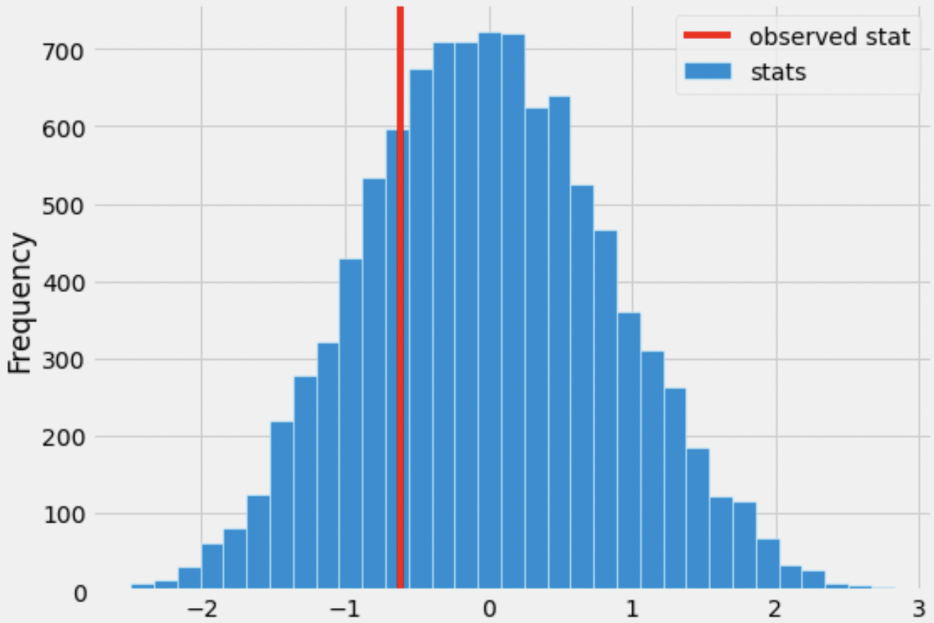
Roughly one-quarter of the area of the histogram above is to the left of the red line. What is the correct interpretation of this result?
There is roughly a one quarter probability that Kelsey Plum’s number of assists in winning games and in losing games come from the same distribution.
The significance level of this hypothesis test is roughly a quarter.
Under the assumption that Kelsey Plum’s number of assists in winning games and in losing games come from the same distribution, and that she wins 22 of the 31 games she plays, the chance of her averaging at least 0.61 more assists in wins than losses is roughly a quarter.
Under the assumption that Kelsey Plum’s number of assists in winning games and in losing games come from the same distribution, and that she wins 22 of the 31 games she plays, the chance of her averaging 0.61 more assists in wins than losses is roughly a quarter.
Answer: Under the assumption that Kelsey Plum’s number of assists in winning games and in losing games come from the same distribution, and that she wins 22 of the 31 games she plays, the chance of her averaging at least 0.61 more assists in wins than losses is roughly a quarter. (Option 3)
First, we should note that the area to the left of the red line (a quarter) is the p-value of our hypothesis test. Generally, the p-value is the probability of observing an outcome as or more extreme than the observed, under the assumption that the null hypothesis is true. The direction to look in depends on the alternate hypothesis; here, since our alternative hypothesis is that the number of assists Kelsey Plum makes in winning games is higher on average than in losing games, a “more extreme” outcome is where the assists in winning games are higher than in losing games, i.e. where \text{(assists in wins)} - \text{(assists in losses)} is positive or where \text{(assists in losses)} - \text{(assists in wins)} is negative. As mentioned in the solution to the first subpart, our test statistic is \text{(assists in losses)} - \text{(assists in wins)}, so a more extreme outcome is one where this is negative, i.e. to the left of the observed statistic.
Let’s first rule out the first two options.
Now, the only difference between Options 3 and 4 is the inclusion of “at least” in Option 3. Remember, to compute a p-value we must compute the probability of observing something as or more extreme than the observed, under the null. The “or more” corresponds to “at least” in Option 3. As such, Option 3 is the correct choice.
The average score on this problem was 70%.
True or False: The histogram drawn in the previous subpart is a density histogram.
True
False
Answer: False
The area of a density histogram is 1. The area of the histogram drawn in the previous subpart is much larger than 1. In fact, the area of this histogram is in the hundreds or thousands; you can draw a rectangle stretching from -1 to 1 on the x-axis and 0 to 300 on the y-axis that has area 2 \cdot 300 = 600, and this rectangle is much smaller than the larger histogram.
The average score on this problem was 82%.
Recall, plum has 31 rows.
Consider the function df_choice, defined below.
def df_choice(df):
return df[np.random.choice([True, False], df.shape[0], replace=True)]Suppose we call df_choice(plum) once. What is the
probability that the result is an empty DataFrame?
0
1
\frac{1}{2^{25}}
\frac{1}{2^{30}}
\frac{1}{2^{31}}
\frac{2^{31} - 1}{2^{31}}
\frac{31}{2^{30}}
\frac{31}{2^{31}}
None of the above
Answer: \frac{1}{2^{31}}
First, let’s understand what df_choice does. It takes in
one input, df. The line
np.random.choice([True, False], df.shape[0], replace=True)
evaluates to an array such that:
df (so if df has 31 rows, the output array
will have length 31)True or
False, since the sequence we are selecting from is
[True, False] and we are selecting with replacementSo
np.random.choice([True, False], df.shape[0], replace=True)
is an array the same length as df, with each element
randomly set to True or False. Note that there
is a \frac{1}{2} chance the first
element is True, a \frac{1}{2} chance the second element is
True, and so on.
Then,
df[np.random.choice([True, False], df.shape[0], replace=True)]
is using Boolean indexing to keep only the rows in df where
the array
np.random.choice([True, False], df.shape[0], replace=True)
contains the value True. So, the function
df_choice returns a DataFrame containing
somewhere between 0 and df.shape[0] rows. Note that there
is a \frac{1}{2} chance that the new
DataFrame contains the first row from df, a \frac{1}{2} chance that the new DataFrame
contains the second row from df, and so on.
In this question, the only input ever given to df_choice
is plum, which has 31 rows.
In this subpart, we’re asked for the probability that
df_choice(plum) is an empty DataFrame. There are 31 rows,
and each of them have a \frac{1}{2}
chance of being included in the output, and so a \frac{1}{2} chance of being missing. So, the
chance that they are all missing is:
\begin{aligned} P(\text{empty DataFrame}) &= P(\text{all rows missing}) \\ &= P(\text{row 0 missing and row 1 missing and ... and row 30 missing}) \\ &= P(\text{row 0 missing}) \cdot P(\text{row 1 missing}) \cdot ... \cdot P(\text{row 30 missing}) \\ &= \frac{1}{2} \cdot \frac{1}{2} \cdot ... \cdot \frac{1}{2} \\ &= \boxed{\frac{1}{2^{31}}} \end{aligned}
The average score on this problem was 83%.
Suppose we call df_choice(plum) once. What is the
probability that the result is a DataFrame with 30 rows?
0
1
\frac{1}{2^{25}}
\frac{1}{2^{30}}
\frac{1}{2^{31}}
\frac{2^{31} - 1}{2^{31}}
\frac{31}{2^{30}}
\frac{31}{2^{31}}
None of the above
Answer: \frac{31}{2^{31}}
In order for the resulting DataFrame to have 30 rows, exactly 1 row must be missing, and the other 30 must be present.
To start, let’s consider one row in particular, say, row 7. The probability that row 7 is missing is \frac{1}{2}, and the probability that rows 0 through 6 and 8 through 30 are all present is \frac{1}{2} \cdot \frac{1}{2} \cdot ... \cdot \frac{1}{2} = \frac{1}{2^{30}} using the logic from the previous subpart. So, the probability that row 7 is missing AND all other rows are present is \frac{1}{2} \cdot \frac{1}{2^{30}} = \frac{1}{2^{31}}.
Then, in order for there to be 30 rows, either row 0 must be missing, or row 1 must be missing, and so on:
\begin{aligned} P(\text{exactly one row missing}) &= P(\text{only row 0 is missing or only row 1 is missing or ... or only row 30 is missing}) \\ &= P(\text{only row 0 is missing}) + P(\text{only row 1 is missing}) + ... + P(\text{only row 30 is missing}) \\ &= \frac{1}{2^{31}} + \frac{1}{2^{31}} + ... + \frac{1}{2^{31}} \\ &= \boxed{\frac{31}{2^{31}}} \end{aligned}
The average score on this problem was 48%.
Suppose we call df_choice(plum) once.
True or False: The probability that the result is a
DataFrame that consists of just row 0 from
plum (and no other rows) is equal to the probability you
computed in the first subpart of this problem.
True
False
Answer: True
An important realization to make is that all subsets
of the rows in plum are equally likely to be returned by
df_choice(plum), and they all have probability \frac{1}{2^{31}}. For instance, one subset of
plum is the subset where rows 2, 5, 8, and 30 are missing,
and the rest are all present. The probability that this subset is
returned by df_choice(plum) is \frac{1}{2^{31}}.
This is true because for each individual row, the probability that it is present or missing is the same – \frac{1}{2} – so the probability of any subset is a product of 31 \frac{1}{2}s, which is \frac{1}{2^{31}}. (The answer to the previous subpart was not \frac{1}{2^{31}} because it was asking about multiple subsets – the subset where only row 0 was missing, and the subset where only row 1 was missing, and so on).
So, the probability that df_choice(plum) consists of
just row 0 is \frac{1}{2^{31}}, and
this is the same as the answer to the first subpart (\frac{1}{2^{31}}); in both situations, we are
calculating the probability of one specific subset.
The average score on this problem was 63%.
Suppose we call df_choice(plum) once.
What is the probability that the resulting DataFrame has 0 rows, or 1 row, or 30 rows, or 31 rows?
0
1
\frac{1}{2^{25}}
\frac{1}{2^{30}}
\frac{1}{2^{31}}
\frac{2^{31} - 1}{2^{31}}
\frac{31}{2^{30}}
\frac{31}{2^{31}}
None of the above
Answer: \frac{1}{2^{25}}
Here, we’re not being asked for the probability of one specific subset (like the subset containing just row 0); rather, we’re being asked for the probability of various different subsets, so our calculation will be a bit more involved.
We can break our problem down into four pieces. We can find the probability that there are 0 rows, 1 row, 30 rows, and 31 rows individually, and add these probabilities up, since only one of them can happen at a time (it’s impossible for a DataFrame to have both 1 and 30 rows at the same time; these events are “mutually exclusive”). It turns out we’ve already calculated two of these probabilities:
The other two possibilities are symmetric with the above two!
Putting it all together, we have:
\begin{aligned} P(\text{number of returned rows is 0, 1, 30, or 31}) &= P(\text{0 rows are returned}) + P(\text{1 row is returned}) + P(\text{30 rows are returned}) + P(\text{31 rows are returned}) \\ &= \frac{1}{2^{31}} + \frac{31}{2^{31}} + \frac{31}{2^{31}} + \frac{1}{2^{31}} \\ &= \frac{1 + 31 + 31 + 1}{2^{31}} \\ &= \frac{64}{2^{31}} \\ &= \frac{2^6}{2^{31}} \\ &= \frac{1}{2^{31 - 6}} \\ &= \boxed{\frac{1}{2^{25}}} \end{aligned}
The average score on this problem was 35%.
In addition to the plum DataFrame, we also have access
to the season DataFrame, which contains statistics on all
players in the WNBA in the 2021 season. The first few rows of
season are shown below. (Remember to keep the data
description from the top of the exam open in another tab!)
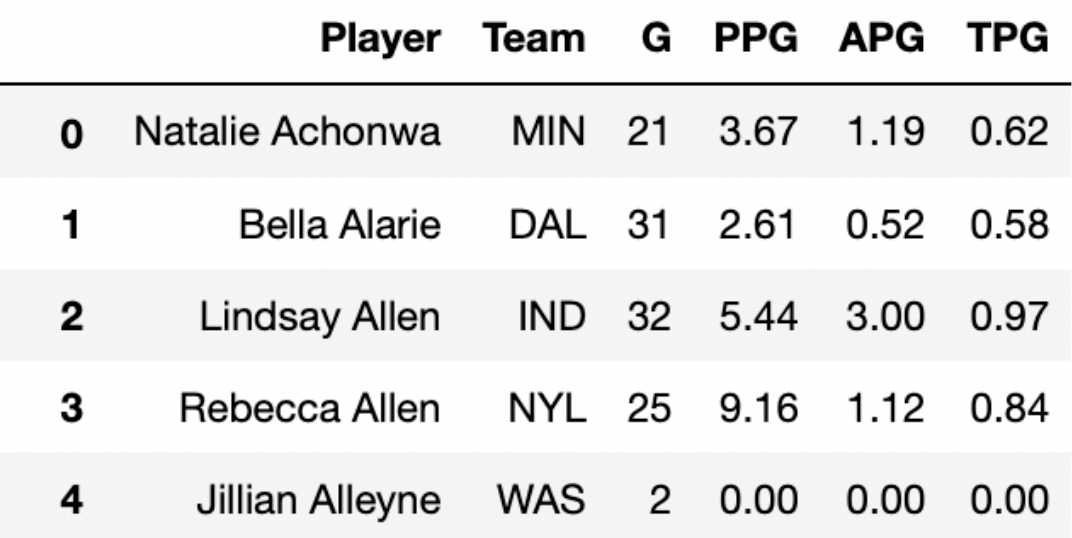
Each row in season corresponds to a single player. For
each player, we have: - 'Player' (str), their
name - 'Team' (str), the three-letter code of
the team they play on - 'G' (int), the number
of games they played in the 2021 season - 'PPG'
(float), the number of points they scored per game played -
'APG' (float), the number of assists (passes)
they made per game played - 'TPG' (float), the
number of turnovers they made per game played
Note that all of the numerical columns in season must
contain values that are greater than or equal to 0.
Which of the following is the best choice for the index of
season?
'Player'
'Team'
'G'
'PPG'
Answer: 'Player'
Ideally, the index of a DataFrame is unique, so that we can use it to
“identify” the rows. Here, each row is about a player, so
'Player' should be the index. 'Player' is the
only column that is likely to be unique; it is possible that two players
have the same name, but it’s still a better choice of index
than the other three options, which are definitely not unique.
The average score on this problem was 95%.
Note: For the rest of the exam, assume that the
index of season is still 0, 1, 2, 3, …
Below is a histogram showing the distribution of the number of
turnovers per game for all players in season.
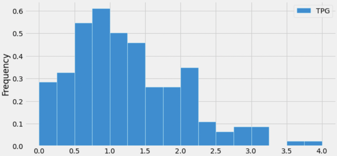
Suppose, throughout this question, that the mean number of turnovers per game is 1.25. Which of the following is closest to the median number of turnovers per game?
0.5
0.75
1
1.25
1.5
1.75
Answer: 1
The median of a distribution is the value that is “halfway” through the distribution, i.e. the value such that half of the values in the distribution are larger than it and half the values in the distribution are smaller than it.
Visually, we’re looking for the location on the x-axis where we can draw a vertical line that splits the area of the histogram in half. While it’s impossible to tell the exact median of the distribution, since we don’t know how the values are distributed within the bars, we can get pretty close by using this principle.
Immediately, we can rule out 0.5, 0.75, 1.5, and 1.75, since they are too far from the “center” of the distribution (imagine drawing vertical lines at any of those points on the x-axis; they don’t split the distribution’s area in half). To decide between 1 and 1.25, we can use the fact that the distribution is right-skewed, meaning that its mean is larger than its median (intuitively, the mean is dragged in the direction of the tail, which is to the right). This means that the median should be less than the mean. We are given that the mean of the distribution is 1.25, so the median should be 1.
The average score on this problem was 73%.
Sabrina Ionescu and Sami Whitcomb are both players on the New York Liberty, and are both California natives.
In “original units”, Sabrina Ionescu had 3.5 turnovers per game. In standard units, her turnovers per game is 3.
In standard units, Sami Whitcomb’s turnovers per game is -1. How many turnovers per game did Sami Whitcomb have in original units? Round your answer to 3 decimal places.
Note: You will need the fact from the previous subpart that the mean number of turnovers per game is 1.25.
Answer: 0.5
To convert a value x to standard units (denoted by x_{\text{su}}), we use the following formula:
x_{\text{su}} = \frac{x - \text{mean of }x}{\text{SD of }x}
Let’s look at the first line given to us: In “original units”, Sabrina Ionescu had 3.5 turnovers per game. In standard units, her turnovers per game is 3.
Substituting the information we know into the above equation gives us:
3 = \frac{3.5 - 1.25}{\text{SD of }x}
In order to convert future values from original units to standard units, we’ll need to know \text{SD of }x, which we don’t currently but can obtain by rearranging the above equation. Doing so yields
\text{SD of }x = \frac{3.5-1.25}{3} = \frac{2.25}{3} = 0.75
Now, let’s look at the second line we’re given: In standard units, Sami Whitcomb’s turnovers per game is -1. How many turnovers per game did Sami Whitcomb have in original units? Round your answer to 3 decimal places.
We have all the information we need to convert Sami Whitcomb’s turnovers per game from standard units to original units! Plugging in the values we know gives us:
\begin{aligned} x_{\text{su}} &= \frac{x - \text{mean of }x}{\text{SD of }x} \\ -1 &= \frac{x - 1.25}{0.75} \\ -0.75 &= x - 1.25 \\ 1.25 - 0.75 &= x \\ x &= \boxed{0.5} \end{aligned}
Thus, in original units, Sami Whitcomb averaged 0.5 turnovers per game.
The average score on this problem was 87%.
What is the smallest possible number of turnovers per game, in standard units? Round your answer to 3 decimal places.
Answer: -1.667
The smallest possible number of turnovers per game in original units is 0 (which a player would have if they never had a turnover – that would mean they’re really good!). To find the smallest possible turnovers per game in standard units, all we need to do is convert 0 from original units to standard units. This will involve our work from the previous subpart.
\begin{aligned} x_{\text{su}} &= \frac{x - \text{mean of }x}{\text{SD of }x} \\ &= \frac{0 - 1.25}{0.75} \\ &= -\frac{1.25}{0.75} \\ &= -\frac{5}{3} = \boxed{-1.667} \end{aligned}
The average score on this problem was 82%.
Let’s switch our attention to the relationship between the number of
points per game and the number of assists per game for all players in
season. Using season, we compute the following
information:
Let’s start by using points per game (x) to predict assists per game (y).
Tina Charles had 27 points per game in 2021, the most of any player in the WNBA. What is her predicted assists per game, according to the regression line? Round your answer to 3 decimal places.
Answer: 5.4
We need to find and use the regression line to find the predicted y for an x of 27. There are two ways to proceed:
Both solutions work; for the sake of completeness, we’ll show both. Recall, r is the correlation coefficient between x and y, which we are told is 0.65.
Solution 1:
First, we need to convert 27 points per game to standard units. Doing so yields
x_{\text{su}} = \frac{x - \text{mean of }x}{\text{SD of }x} = \frac{27 - 7}{5} = 4
Per the regression line, y_\text{su} = r \cdot x_\text{su}, we have y_\text{su} = 0.65 \cdot 4 = 2.6, which is Tina Charles’ predicted assists per game in standard units. All that’s left is to convert this value back to original units:
\begin{aligned} y_{\text{su}} &= \frac{y - \text{mean of }y}{\text{SD of }y} \\ 2.6 &= \frac{y - 1.5}{1.5} \\ 2.6 \cdot 1.5 + 1.5 &= y \\ y &= \boxed{5.4} \end{aligned}
So, the regression line predicts Tina Charles will have 5.4 assists per game (in original units).
Solution 2:
First, we need to find the slope m and intercept b:
m = r \cdot \frac{\text{SD of }y }{\text{SD of }x} = 0.65 \cdot \frac{1.5}{5} = 0.195
b = \text{mean of }y - m \cdot \text{mean of }x = 1.5 - 0.195 \cdot 7 = 0.135
Then,
y = mx + b \implies y = 0.195 \cdot 27 + 0.135 = \boxed{5.4}
So, once again, the regression line predicts Tina Charles will have 5.4 assists per game.
Note: The numbers in this problem may seem ugly, but students taking this exam had access to calculators since this exam was online. It also turns out that the numbers were easier to work with in Solution 1 over Solution 2; this was intentional.
The average score on this problem was 81%.
Tina Charles actually had 2.1 assists per game in the 2021 season.
What is the error, or residual, for the prediction in the previous subpart? Round your answer to 3 decimal places.
Answer: -3.3
Residuals are defined as follows:
\text{residual} = \text{actual } y - \text{predicted }y
2.1 - 5.4 = -3.3, which gives us our answer.
Note: Many students answered 3.3. Pay attention to the order of the calculation!
The average score on this problem was 82%.
Select all true statements below regarding the regression line between points per game (x) and assists per game (y).
The point (0, 0) is guaranteed to be on the regression line when both x and y are in standard units.
The point (0, 0) is guaranteed to be on the regression line when both x and y are in original units.
The point (7, 1.5) is guaranteed to be on the regression line when both x and y are in standard units.
The point (7, 1.5) is guaranteed to be on the regression line when both x and y are in original units.
None of the above
Answers:
The main idea being assessed here is the fact that the point (\text{mean of }x, \text{mean of }y) always lies on the regression line. Indeed, in original units, 7 is the average x (PPG) and 1.5 is the average y (APG); this information was provided to us at the start of the problem. The nuance behind this problem lies in the units that are being used in the regression line.
When the regression line is in standard units:
When the regression line is in original units:
y = mx + b = mx + \text{mean of }y - m \cdot \text{mean of }x
The average score on this problem was 87%.
So far, we’ve been using points per game (x) to predict assists per game (y). Suppose we found the regression line (when both x and y are in original units) to be y = ax + b.
Now, let’s reverse x and y. That is, we will now use assists per game (x) to predict points per game (y). The resulting regression line (when both x and y are in original units) is y = cx + d.
Which of the following statements is guaranteed to be true?
a = c
a > c
a < c
Using just the information given in this problem, it is impossible to determine the relationship between a and c.
Answer: a < c
The formula for the slope of the regression line is m = r \cdot \frac{\text{SD of }y}{\text{SD of }x}. Note that the correlation coefficient r is symmetric, meaning that the correlation between x and y is the same as the correlation between y and x.
In the two regression lines mentioned in this problem, we have
\begin{aligned} a &= r \cdot \frac{\text{SD of assists per game}}{\text{SD of points per game}} \\ c &= r \cdot \frac{\text{SD of points per game}}{\text{SD of assists per game}} \end{aligned}
We’re told in the problem that the SD of points per game is 5 and the SD of assists per game is 1.5. So, a = r \cdot \frac{1.5}{5} and c = r \cdot \frac{5}{1.5}; since \frac{1.5}{5} < \frac{5}{1.5}, a < c.
The average score on this problem was 74%.
Recall that the mean points per game is 7, with a standard deviation of 5. Also note that for all players, points per game must be greater than or equal to 0.
Using Chebyshev’s inequality, we find that at least p\% of players scored 25 or fewer points per game.
What is the value of p? Give your answer as number between 0 and 100, rounded to 3 decimal places.
Answer: 92.284\%
Recall, Chebyshev’s inequality states that the proportion of values within z standard deviations of the mean is at least 1 - \frac{1}{z^2}.
To approach the problem, we’ll start by converting 25 points per game to standard units. Doing so yields \frac{25 - 7}{5} = 3.6. This means that 25 is 3.6 standard deviations above the mean. The value 3.6 standard deviations below the mean is 7 - 3.6 \cdot 5 = -11, so when we use Chebyshev’s inequality with z = 3.6, we will get a lower bound on the proportion of values between -11 and 25. However, as the question tells us, points per game must be non-negative, so in this case the proportion of values between -11 and 25 is the same as the proportion of values between 0 and 25 (i.e. the proportion of values less than or equal to 25).
When z = 3.6, we have 1 - \frac{1}{z^2} = 1 - \frac{1}{3.6^2} = 0.922839, which as a percentage rounded to three decimal places is 92.284\%. Thus, at least 92.284\% scored 25 or fewer points per game.
The average score on this problem was 46%.
Note: This problem is out of scope; it covers material no longer included in the course.
Note: This question uses the mathematical definition
of percentile, not np.percentile.
The array aces defined below contains the points per
game scored by all members of the Las Vegas Aces. Note that it contains
14 numbers that are in sorted order.
aces = np.array([0, 0, 1.05, 1.47, 1.96, 2, 3.25,
                 10.53, 11.09, 11.62, 12.19,
                 14.24, 14.81, 18.25])
As we saw in lab, percentiles are not unique. For instance, the
number 1.05 is both the 15th percentile and 16th percentile of
aces.
There is a positive integer q,
between 0 and 100, such that 14.24 is the qth percentile of aces, but
14.81 is the (q+1)th percentile of
aces.
What is the value of q? Give your answer as an integer between 0 and 100.
Answer: 85
For reference, recall that we find the pth percentile of a collection of n numbers as follows:
h = \frac{p}{100} \cdot n
If h is an integer, define k = h. Otherwise, let k be the smallest integer greater than h.
Take the kth element of the sorted collection (start counting from 1, not 0).
To start, it’s worth emphasizing that there are n = 14 numbers in aces total.
14.24 is at position 12 (when the positions are numbered 1 through
14).
Let’s try and find a value of p such that 14.24 is the pth percentile. To do so, we might try and find what “percentage” of the way through the distribution 14.24 is; doing so gives \frac{12}{14} = 85.71\%. If we follow the process outlined above with p = 85, we get that h = \frac{85}{100} \cdot 14 = 11.9 and thus k = 12, meaning that the 85th percentile is the number at position 12, which 14.24.
Let’s see what happens when we try the same process with p = 86. This time, we have h = \frac{86}{100} \cdot 14 = 12.04 and thus k = 13, meaning that the 86th percentile is the number at position 13, which is 14.81.
This means that the value of q is 85 – the 85th percentile is 14.24, while the 86th percentile is 14.81.
The average score on this problem was 57%.
For your convenience, we show the first few rows of
season again below.
In the past three problems, we presumed that we had access to the
entire season DataFrame. Now, suppose we only have access
to the DataFrame small_season, which is a random sample of
size 36 from season. We’re interested in
learning about the true mean points per game of all players in
season given just the information in
small_season.
To start, we want to bootstrap small_season 10,000 times
and compute the mean of the resample each time. We want to store these
10,000 bootstrapped means in the array boot_means.
Here is a broken implementation of this procedure.
boot_means = np.array([])
for i in np.arange(10000):
    resample = small_season.sample(season.shape[0], replace=False)  # Line 1
    resample_mean = small_season.get('PPG').mean()                  # Line 2
    np.append(boot_means, new_mean)                                 # Line 3
For each of the 3 lines of code above (marked by comments), specify what is incorrect about the line by selecting one or more of the corresponding options below. Or, select “Line _ is correct as-is” if you believe there’s nothing that needs to be changed about the line in order for the above code to run properly.
What is incorrect about Line 1? Select all that apply.
Currently the procedure samples from small_season, when
it should be sampling from season
The sample size is season.shape[0], when it should be
small_season.shape[0]
Sampling is currently being done without replacement, when it should be done with replacement
Line 1 is correct as-is
Answers:
season.shape[0], when it should be
small_season.shape[0]Here, our goal is to bootstrap from small_season. When
bootstrapping, we sample with replacement from our
original sample, with a sample size that’s equal to the original
sample’s size. Here, our original sample is small_season,
so we should be taking samples of size
small_season.shape[0] from it.
Option 1 is incorrect; season has nothing to do with
this problem, as we are bootstrapping from
small_season.
The average score on this problem was 95%.
What is incorrect about Line 2? Select all that apply.
Currently it is taking the mean of the 'PPG' column in
small_season, when it should be taking the mean of the
'PPG' column in season
Currently it is taking the mean of the 'PPG' column in
small_season, when it should be taking the mean of the
'PPG' column in resample
.mean() is not a valid Series method, and should be
replaced with a call to the function np.mean
Line 2 is correct as-is
Answer: Currently it is taking the mean of the
'PPG' column in small_season, when it should
be taking the mean of the 'PPG' column in
resample
The current implementation of Line 2 doesn’t use the
resample at all, when it should. If we were to leave Line 2
as it is, all of the values in boot_means would be
identical (and equal to the mean of the 'PPG' column in
small_season).
Option 1 is incorrect since our bootstrapping procedure is
independent of season. Option 3 is incorrect because
.mean() is a valid Series method.
The average score on this problem was 98%.
What is incorrect about Line 3? Select all that apply.
The result of calling np.append is not being reassigned
to boot_means, so boot_means will be an empty
array after running this procedure
The indentation level of the line is incorrect –
np.append should be outside of the for-loop
(and aligned with for i)
new_mean is not a defined variable name, and should be
replaced with resample_mean
Line 3 is correct as-is
Answers:
np.append is not being reassigned
to boot_means, so boot_means will be an empty
array after running this procedurenew_mean is not a defined variable name, and should be
replaced with resample_meannp.append returns a new array and does not modify the
array it is called on (boot_means, in this case), so Option
1 is a necessary fix. Furthermore, Option 3 is a necessary fix since
new_mean wasn’t defined anywhere.
Option 2 is incorrect; if np.append were outside of the
for-loop, none of the 10,000 resampled means would be saved
in boot_means.
The average score on this problem was 94%.
Suppose we’ve now fixed everything that was incorrect about our bootstrapping implementation.
Recall from earlier in the exam that, in season, the
mean number of points per game is 7, with a standard deviation of 5.
It turns out that when looking at just the players in
small_season, the mean number of points per game is 9, with
a standard deviation of 4. Remember that small_season is a
random sample of size 36 taken from season.
Which of the following histograms visualizes the empirical distribution of the sample mean, computed using the bootstrapping procedure above?
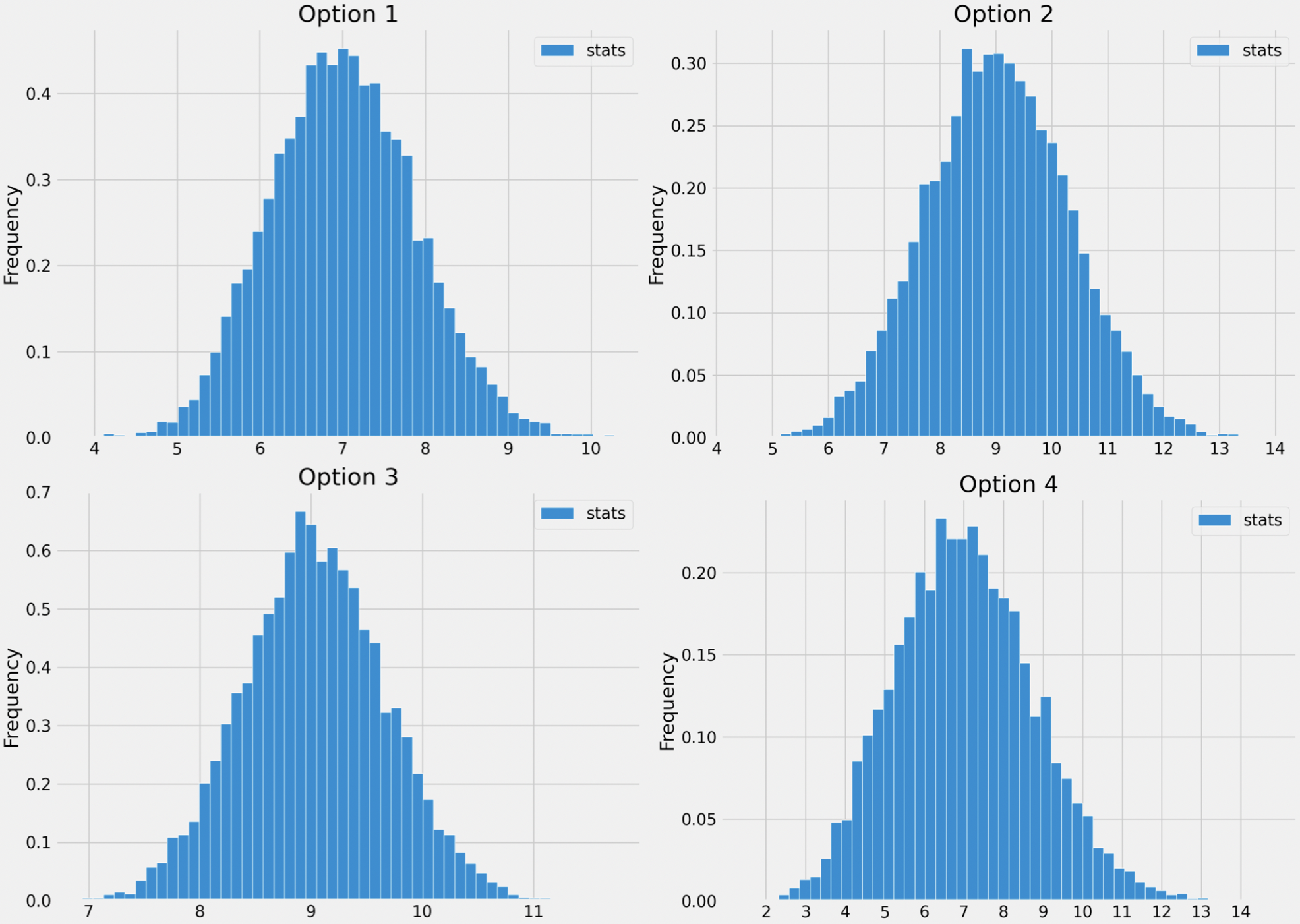
Option 1
Option 2
Option 3
Option 4
Answer: Option 3
The key to this problem is knowing to use the Central Limit Theorem. Specifically, we know that if we collect many samples from a population with replacement, then the distribution of the sample means will be roughly normal with:
Here, the “population” is small_season,
because that is the sample we’re repeatedly (re)sampling from. While
season is actually the population, it is not seen at all in
the bootstrapping process, so it doesn’t directly influence the
distribution of the bootstrapped sample means.
The mean of small_season is 9, and so is the
distribution of bootstrapped sample means. The standard deviation of
small_season is 4, so the square root law, the standard
deviation of the distribution of bootstrapped sample means is \frac{4}{\sqrt{36}} = \frac{4}{6} =
\frac{2}{3}.
The answer now boils down to choosing the histogram that looks roughly normally distributed with a mean of 9 and a standard deviation of \frac{2}{3}. Options 1 and 4 can be ruled out right away since their means seem to be smaller than 9. To decide between Options 2 and 3, we can use the inflection point rule, which states that in a normal distribution, the inflection points occur at one standard deviation above and one standard deviation below the mean. (An inflection point is when a curve changes from opening upwards to opening downwards.) See the picture below for more details.
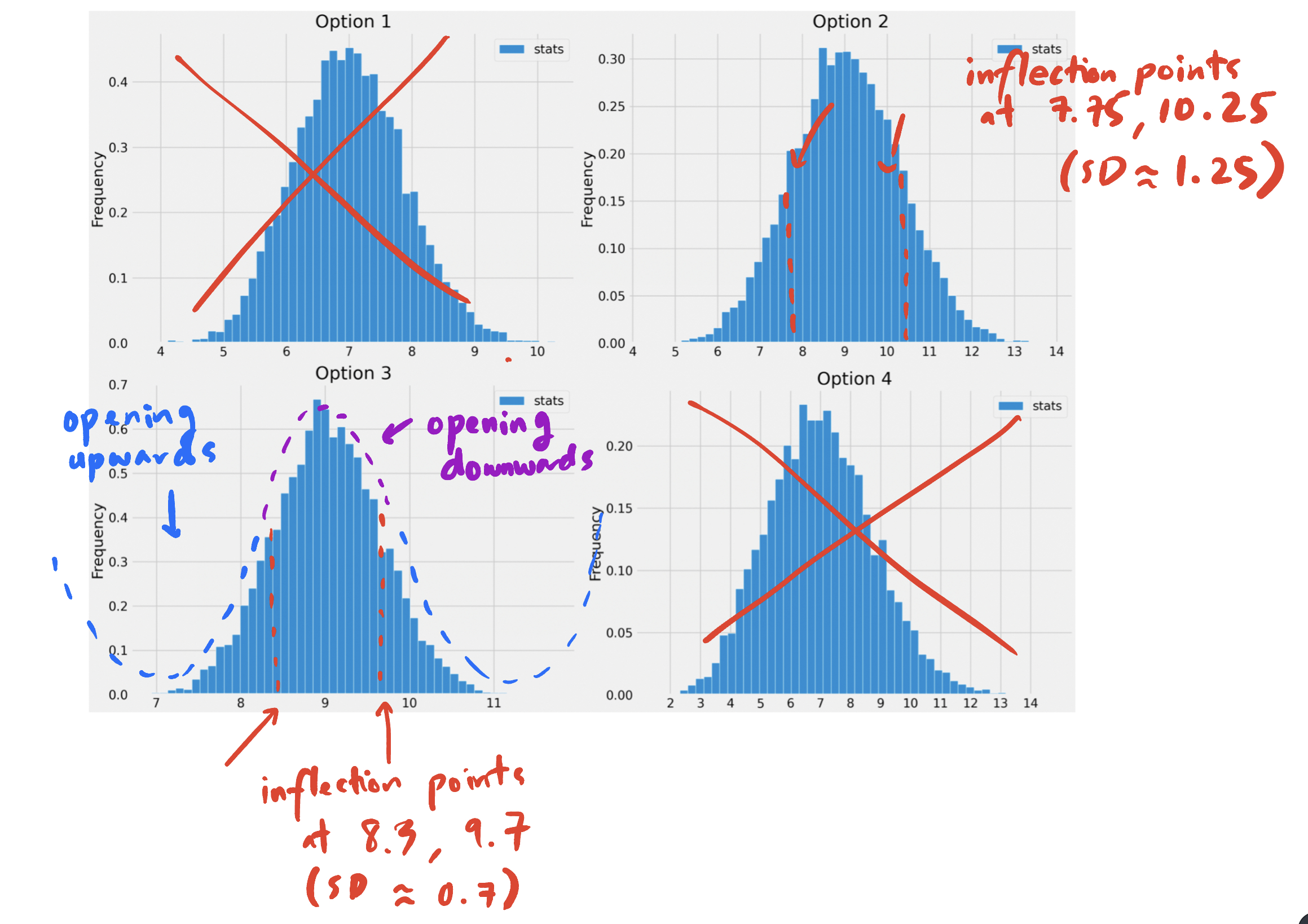
Option 3 is the only distribution that appears to be centered at 9 with a standard deviation of \frac{2}{3} (0.7 is close to \frac{2}{3}), so it must be the empirical distribution of the bootstrapped sample means.
The average score on this problem was 42%.
We construct a 95% confidence interval for the true mean points per game for all players by taking the middle 95% of the bootstrapped sample means.
left_b = np.percentile(boot_means, 2.5)
right_b = np.percentile(boot_means, 97.5)
boot_ci = [left_b, right_b]
Select the most correct statement below.
(left_b + right_b) / 2 is exactly equal to the mean
points per game in season.
(left_b + right_b) / 2 is not necessarily equal to the
mean points per game in season, but is close.
(left_b + right_b) / 2 is exactly equal to the mean
points per game in small_season.
(left_b + right_b) / 2 is not necessarily equal to the
mean points per game in small_season, but is close.
(left_b _+ right_b) / 2 is not close to either the mean
points per game in season or the mean points per game in
small_season.
Answer: (left_b + right_b) / 2 is not
necessarily equal to the mean points per game in
small_season, but is close.
Normal-based confidence intervals are of the form [\text{mean} - \text{something}, \text{mean} + \text{something}]. In such confidence intervals, it is the case that the average of the left and right endpoints is exactly the mean of the distribution used to compute the interval.
However, the confidence interval we’ve created is not normal-based, rather it is bootstrap-based! As such, we can’t say that anything is exactly true; this rules out Options 1 and 3.
Our 95% confidence interval was created by taking the middle 95% of
bootstrapped sample means. The distribution of bootstrapped sample means
is roughly normal, and the normal distribution is
symmetric (the mean and median are both equal, and represent the
“center” of the distribution). This means that the middle of our 95%
confidence interval should be roughly equal to the mean of the
distribution of bootstrapped sample means. This implies that Option 4 is
correct; the difference between Options 2 and 4 is that Option 4 uses
small_season, which is the sample we bootstrapped from,
while Option 2 uses season, which was not accessed at all
in our bootstrapping procedure.
The average score on this problem was 62%.
Instead of bootstrapping, we could also construct a 95% confidence interval for the true mean points per game by using the Central Limit Theorem.
Recall that, when looking at just the players in
small_season, the mean number of points per game is 9, with
a standard deviation of 4. Also remember that small_season
is a random sample of size 36 taken from season.
Using only the information that we have about
small_season (i.e. without using any facts about
season), compute a 95% confidence interval for the true
mean points per game.
What are the left and right endpoints of your interval? Give your answers as numbers rounded to 3 decimal places.
Answer: [7.667, 10.333]
In a normal distribution, roughly 95% of values are within 2 standard deviations of the mean. The CLT tells us that the distribution of sample means is roughly normal, and in subpart 4 of this problem we already computed the SD of the distribution of sample means to be \frac{2}{3}.
So, our normal-based 95% confidence interval is computed as follows:
\begin{aligned} &[\text{mean of sample} - 2 \cdot \text{SD of distribution of sample means}, \text{mean of sample} + 2 \cdot \text{SD of distribution of sample means}] \\ &= [9 - 2 \cdot \frac{4}{\sqrt{36}}, 9 + 2 \cdot \frac{4}{\sqrt{36}}] \\ &= [9 - \frac{4}{3}, 9 + \frac{4}{3}] \\ &\approx \boxed{[7.667, 10.333]} \end{aligned}
The average score on this problem was 87%.
Recall that the mean points per game in season is 7,
which is not in the interval you found above (if it is, check your
work!).
Select the true statement below.
The 95% confidence interval we created in the previous subpart did not contain the true mean points per game, which means that the distribution of the sample mean is not normal.
The 95% confidence interval we created in the previous subpart did
not contain the true mean points per game, which means that the
distribution of points per game in small_season is not
normal.
The 95% confidence interval we created in the previous subpart did not contain the true mean points per game. This is to be expected, because the Central Limit Theorem is only correct 95% of the time.
The 95% confidence interval we created in the previous subpart did not contain the true mean points per game, but if we collected many original samples and constructed many 95% confidence intervals, then roughly 95% of them would contain the true mean points per game.
The 95% confidence interval we created in the previous subpart did not contain the true mean points per game, but if we collected many original samples and constructed many 95% confidence intervals, then exactly 95% of them would contain the true mean points per game.
Answer: The 95% confidence interval we created in the previous subpart did not contain the true mean points per game, but if we collected many original samples and constructed many 95% confidence intervals, then roughly 95% of them would contain the true mean points per game.
In a confidence interval, the confidence level gives us a level of confidence in the process used to create the confidence interval. If we repeat the process of collecting a sample from the population and using the sample to construct a c% confidence interval for the population mean, then roughly c% of the intervals we create should contain the population mean. Option 4 is the only option that corresponds to this interpretation; the others are all incorrect in different ways.
The average score on this problem was 87%.
Note: This problem is out of scope; it covers material no longer included in the course.
The WNBA is interested in helping boost their players’ social media presence, and considers various ways of making that happen.
Which of the following claims can be tested using a randomized controlled trial? Select all that apply.
Winning two games in a row causes a player to gain Instagram followers.
Drinking Gatorade causes a player to gain Instagram followers.
Playing for the Las Vegas Aces causes a player to gain Instagram followers.
Deleting Twitter causes a player to gain Instagram followers.
None of the above.
Answers:
The key to this problem is understanding the nature of randomized controlled trials (RCTs). To run an RCT, we must be able to randomly assign our test subjects to either a treatment or control group, and apply some treatment only to the treatment group. With that in mind, let’s look at the four options.
Note, our assessment above did not look at the outcome, gaining Instagram followers, at all. While to us it may seem unlikely that drinking Gatorade causes a player to gain Instagram followers, that doesn’t mean we can’t run an RCT to check.
The average score on this problem was 77%.