← return to practice.dsc10.com
Instructor(s): Janine Tiefenbruck
This exam was administered in-person. The exam was closed-notes, except students were provided a copy of the DSC 10 Reference Sheet. No calculators were allowed. Students had 3 hours to take this exam.
⚠️ PDF version available here .
Note (groupby / pandas 2.0): Pandas 2.0+ no longer
silently drops columns that can’t be aggregated after a
groupby, so code written for older pandas may behave
differently or raise errors. In these practice materials we use
.get() to select the column(s) we want after
.groupby(...).mean() (or other aggregations) so that our
solutions run on current pandas. On real exams you will not be penalized
for omitting .get() when the old behavior would have
produced the same answer.
The Olympic Games are the world’s leading international sporting
event, dating back to ancient Greece. Today, we’ll explore data on
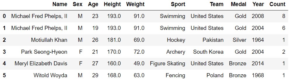
modern Olympic medalists. Each row in the DataFrame
olympians corresponds to a type of medal earned by one
Olympic athlete in one year.
The columns of olympians are as follows:
"Name" (str): The name of the athlete.
Unique for each athlete."Sex" (str): The sex of the athlete,
denoted by “M” or “F”."Age" (int): The age of the athlete at the
time of the Olympics."Height" (float): The height of the
athlete in centimeters."Weight" (float): The weight of the
athlete in kilograms."Sport" (str): The sport in which the
athlete competed."Team" (str): The team or country the
athlete represented."Medal" (str): The type of medal won
(“Gold”, “Silver”, or “Bronze”)."Year" (int): The year of the Olympic
Games."Count" (int): The number of medals of
this type earned by this athlete in this year.The first few rows of olympians are shown below, though
olympians has many more rows than pictured. The data in
olympians is only a sample from the much larger population
of all Olympic medalists.
Throughout this exam, assume that we have already run
import babypandas as bpd and
import numpy as np.
Which of the following columns would be an appropriate index for the
olympians DataFrame?
"Name"
"Sport"
"Team"
None of these.
Answer: None of these.
To decide what an appropriate index would be, we need to keep in mind
that in each row, the index should have a unique value – that is, we
want the index to uniquely identify rows of the DataFrame. In this case,
there will obviously be repeats in "team" and
"sport", since these will appear multiple times for each
Olympic event. Although the name is unique for each athlete, the same
athlete could compete in multiple Olympics (for example, Michael Phelps
competed in both 2008 and 2004). So, none of these options is a valid
index.
The average score on this problem was 74%.
Frank X. Kugler has Olympic medals in three sports (wrestling,
weightlifting, and tug of war), which is more sports than any other
Olympic medalist. Furthermore, his medals for all three of these sports
are included in the olympians DataFrame. Fill in the blanks
below so that the expression below evaluates to
"Frank X. Kugler".
                (olympians.groupby(__(a)__).__(b)__
                          .reset_index()
                          .groupby(__(c)__).__(d)__
                          .sort_values(by="Age", ascending=False)
.index[0])What goes in blank (a)?
Answer: ["Name", "Sport"] or
["Sport", "Name"]
The question wants us to find the name (Frank X. Kugler) who has
records that correspond to three distinct sports. We know that the same
athlete might have multiple records for a distinct sport if they
participated in the same sport for multiple years. Therefore we should
groupby "Name" and "Sport" to create a
DataFrame with unique Name-Sport pairs. This is a DataFrame that
contains the athletes and their sports (for each athlete, their
corresponding sports are distinct). If an athlete participated in 2
sports, for example, they would have 2 rows corresponding to them in the
DataFrame, 1 row for each distinct sport.
The average score on this problem was 75%.
What goes in blank (b)?
Answer: .sum() or .mean()
or .min(), etc.
Any aggregation method applied on df.groupby() would
work. We only want to remove cases in which an athlete participates in
the same sport for multiple years, and get unique name-sport pairs.
Therefore, we don’t care about the aggregated numeric value. Notice
.unique() is not correct because it is not an aggregation
method used on dataframe after grouping by. If you use
.unique(), it will give you “AttributeError:
‘DataFrameGroupBy’ object has no attribute ‘unique’”. However,
.unique() can be used after Series.groupby().
For more info: [link]
(https://pandas.pydata.org/docs/reference/api/pandas.core.groupby.SeriesGroupBy.unique.html)
The average score on this problem was 96%.
What goes in blank (c)?
Answer: "Name"
Now after resetting the index, we have "Name" and
"Sport" columns containing unique name-sport pairs. The
objective is to count how many different sports each Olympian has medals
in. To do that, we groupby "Name" and later use the
.count() method. This would give a new DataFrame that has a
count of how many times each name shows up in our previous DataFrame
with unique name-sport pairs.
The average score on this problem was 81%.
What goes in blank (d)?
Answer: .count()
The .count() method is applied to each group. In this
context, .count() will get the number of entries for each
Olympian across different sports, since the previous steps ensured each
sport per Olympian is uniquely listed (due to the initial groupby on
both "Name" and "Sport"). It does not matter
what we sort_values by, because the
.groupby('Name').count() method will just put a count of
each "Name" in all of the columns, regardless of the column
name or what value was originally in it.
The average score on this problem was 64%.
In olympians, "Weight" is measured in
kilograms. There are 2.2 pounds in 1 kilogram. If we converted
"Weight" to pounds instead, which of the following
quantities would increase?
The mean of the "Weight" distribution.
The standard deviation of the "Weight" distribution.
The proportion of "Weight" values within 3 standard
deviations
The correlation between "Height" and
"Weight".
The slope of the regression line predicting "Weight"
from
The slope of the regression line predicting "Height"
from
Answer: Options 1, 2, and 5 are correct.
"Weight", μ being the mean in kg and σ being the standard
deviation in kg. Once we scale everything by 2.2 to convert from
kilograms to pounds, we have that"Weight" within 3 standard deviations of the mean stays the
same. Intuitively this should make sense because we are scaling
everything by the same amount, so the proportion of points that are a
specific number of standard deviations away from the mean should be the
same, since the standard deviation and mean get scaled as well. So,
option 3 is incorrect."Weight"(kg) in standard
units is \frac{x~i~−μ}{σ}. Similar to
option 3, "Weight"(pounds) in standard units is \frac{2.2x_{i}-2.2μ}{2.2σ} = \frac{2.2}{2.2}
\frac{x_{i} \cdot μ}{σ} = \frac{x_{i} \cdot μ}{σ}. Again, notice
that the equation in pounds ends up the exact same as in kilograms. The
same applies for "Height" in standard units. Since none of
the variables change when measured in standard units, r doesn’t change.
So, option 4 is incorrect."Weight" and
the x-axis representing "Height". We expect that the taller
someone is, the heavier they will be. So we can expect a positive
regression line slope between Weight and Height. When we convert Weight
from kg to pounds, we are scaling every value in "Weight",
making their values increase. When we scale the the weight values
(y-values) to become bigger, we are making the regression slope even
steeper, because an increase in Height (x) now corresponds to an even
larger increase in Weight(y). So, option 5 is correct."Weight" on the x-axis and
"Height" on the y-axis. Since we are increasing the values
of "Height", we can imagine stretching the x-axis’ values
without changing the y-values, which makes the line more flat and
therefore decreases the slope. So, option 6 is incorrect. Another
approach to both 5 and 6 is to utilize the correlation coefficient
r, which is equal to the slope times \frac{σ~y~}{σ~x~}. We know that multiplying a
set values by a value greater than one increases the spread of the data
which increases standard deviation. In option 5, "Weight"
is in the y-axis, and increasing the numerator of the fraction \frac{σ~y~}{σ~x~} increases r. In
option 6, "Weight" is in the x-axis, and increasing the
denominator the fraction \frac{σ~y~}{σ~x~} decreases r.
The average score on this problem was 80%.
The Olympics are held every two years, in even-numbered years, alternating between the Summer Olympics and Winter Olympics. Summer Olympics are held in years that are a multiple of 4 (such as 2024), and Winter Olympics are held in years that are not a multiple of 4 (such as 2022 or 2026).
We want to add a column to olympics that contains either
"Winter" or "Summer" by applying a function
called season as follows:
olympians.assign(Season=olympians.get("Year").apply(season))Which of the following definitions of season is correct?
Select all that apply.
Notes:
We’ll ignore the fact that the 2020 Olympics were rescheduled to 2021 due to Covid.
Recall that the % operator in Python gives the
remainder upon division. For example, 8 % 3 evaluates to
2.
Way 1:
        def season(year):
            if year % 4 == 0:
                return "Summer"
            return "Winter"
Way 2:
        def season(year):
            return "Winter"
            if year % 4 == 0:
                return "Summer"
Way 3:
        def season(year):
            if year % 2 == 0:
                return "Winter"
            return "Summer"
Way 4:
        def season(year):
            if int(year / 4) != year / 4:
                return "Winter"
            return "Summer"
Way 1
Way 2
Way 3
Way 4
Answer: Way 1 and Way 4
return "Winter" line is before the if
statement. Since nothing after a return statement gets executed
(assuming that the return statement gets executed), no matter what the
year is this function will always return “Winter”. So, way 2 is
incorrect.2020 % 2 evaluates to 0. So, way 3 is
incorrect.year / 4 to an integer using int
changes its value. If the two aren’t equal, then we know that
year / 4 wasn’t an integer before casting, which means that
the year isn’t divisible by 4 and we should return
"Winter". If the code inside the if statement doesn’t
execute, then we know that the year is divisible by 4, so we return
“Summer”. So, way 4 is correct.
The average score on this problem was 89%.
In figure skating, skaters move around an ice rink performing a series of skills, such as jumps and spins. Ylesia has been training for the Olympics, and she has a set routine that she plans to perform.
Let’s say that Ylesia performs a skill successfully if she does not
fall during that skill. Each skill comes with its own probability of
success, as some skills are harder and some are easier. Suppose that the
probabilities of success for each skill in Ylesia’s Olympic routine are
stored in an array called skill_success.
For example, if Ylesia’s Olympic routine happened to only contain
three skills, skill_success might be the array with values
0.92, 0.84, 0.92. However, her routine can contain any number of
skills.
Ylesia wants to simulate one Olympic routine to see how many times
she might fall. Fill in the function count_falls below,
which takes as input an array skill_success and returns as
output the number of times Ylesia falls during her Olympic routine.
        def count_falls(skill_success):
            falls = 0
            for p in skill_success:
                result = np.random.multinomial(1, __(a)__)
                falls = __(b)__
return fallsAnswer: (a): [p, 1-p], (b):
falls + result[1] OR (a): [1-p, p], (b):
falls + result[0]
[p, 1-p]
in blank (a).result, with index 0 being how many times she succeeded
(corresponds to p), and index 1 being how many times she fell
(corresponds to 1-p). Since index 1 corresponds to the scenario in which
she falls, in order to correctly increase the number of falls, we add
falls by result[1]. Therefore, blank (b) is
falls + result[1].Likewise, you can change the order with (a): [1-p, p]
and (b): falls + result[0] and it would still correctly
simulate how many times she falls.
The average score on this problem was 59%.
Fill in the blanks below so that prob_no_falls evaluates
to the exact probability of Ylesia performing her entire routine without
falling.
        prob_no_falls = __(a)__
        for p in skill_success:
            prob_no_falls = __(b)__
prob_no_fallsAnswer: (a): 1, (b):
prob_no_falls * p
prob_no_falls. This should be set to 1 because we’re
computing a probability product, and starting with 1 ensures the initial
value doesn’t affect the multiplication of subsequent
probabilities.prob_no_falls by multiplying it by each probability of
success (p) in skill_success. This is because
the probability of Ylesia not falling throughout multiple independent
skills is the product of her not falling during each skill.
The average score on this problem was 72%.
Fill the blanks below so that approx_prob_no_falls
evaluates to an estimate of the probability that Ylesia performs her
entire routine without falling, based on 10,000 trials. Feel free to use
the function you defined in part (a) as part of your solution.
        results = np.array([])
        for i in np.arange(10000):
            results = np.append(results, __(a)__)
        approx_prob_no_falls = __(b)__
approx_prob_no_fallsAnswer:(a): count_falls(skill_success),
(b): np.count_nonzero(results == 0) / 10000, though there
are many other correct solutions
count_falls(skill_success).np.count_nonzero(results == 0) / 10000.
The average score on this problem was 66%.
Suppose we sample 400 rows of olympians
at random without replacement, then generate a 95% CLT-based confidence
interval for the mean age of Olympic medalists based on this sample.
The CLT is stated for samples drawn with replacement, but in practice, we can often use it for samples drawn without replacement. What is it about this situation that makes it reasonable to still use the CLT despite the sample being drawn without replacement?
The sample is much smaller than the population.
The statistic is the sample mean.
The CLT is less computational than bootstrapping, so we don’t need to sample with replacement like we would for bootstrapping.
The population is normally distributed.
The sample standard deviation is similar to the population standard deviation.
Answer: The sample is much smaller than the population.
The Central Limit Theorem (CLT) states that regardless of the shape of the population distribution, the sampling distribution of the sample mean will be approximately normally distributed if the sample size is sufficiently large. The key factor that makes it reasonable to still use the CLT, is the sample size relative to the population size. When the sample size is much smaller than the population size, as in this case where 400 rows of Olympians are sampled from a likely much larger population of Olympians, the effect of sampling without replacement becomes negligible.
The average score on this problem was 47%.
Suppose our 95% CLT-based confidence interval for the mean age of Olympic medalists is [24.9, 26.1]. What was the mean of ages in our sample?
Answer: Mean = 25.5
We calculate the mean by first determining the width of our interval: 26.1 - 24.9 = 1.2, then we divide this width in half to get 0.6 which represents the distance from the mean to each side of the confidence interval. Using this we can find the mean in two ways: 24.9 + 0.6 = 25.5 OR 26.1 - 0.6 = 25.5.
The average score on this problem was 90%.
Suppose our 95% CLT-based confidence interval for the mean age of Olympic medalists is [24.9, 26.1]. What was the standard deviation of ages in our sample?
Answer: Standard deviation = 6
We can calculate the sample standard deviation (sample SD) by using the 95% confidence interval equation:
\text{sample mean} - 2 * \frac{\text{sample SD}}{\sqrt{\text{sample size}}}, \text{sample mean} + 2 * \frac{\text{sample SD}}{\sqrt{\text{sample size}}}.
Choose one of the end points and start plugging in all the information you have/calculated:
25.5 - 2*\frac{\text{sample SD}}{\sqrt{400}} = 24.9 → \text{sample SD} = \frac{(25.5 - 24.9)}{2}*\sqrt{400} = 6.
The average score on this problem was 55%.
In our sample, we have data on 1210 medals for the sport of gymnastics. Of these, 126 were awarded to American gymnasts, 119 were awarded to Romanian gymnasts, and the remaining 965 were awarded to gymnasts from other nations.
We want to do a hypothesis test with the following hypotheses.
Null: American and Romanian gymnasts win an equal share of Olympic gymnastics medals.
Alternative: American gymnasts win more Olympic gymnastics medals than Romanian gymnasts.
Which test statistic could we use to test these hypotheses?
total variation distance between the distribution of medals by country and the uniform distribution
proportion of medals won by American gymnasts
difference in the number of medals won by American gymnasts and the number of medals won by Romanian gymnasts
absolute difference in proportion of medals won by American gymnasts and proportion of medals won by Romanian gymnasts
Answer: difference in the number of medals won by American gymnasts and the number of medals won by Romanian gymnasts
To test this pair of hypotheses, we need a test statistic that is
large when the data suggests that we reject the null hypothesis, and
small when we fail to reject the null. Now let’s look at each
option:
- Option 1: Total variation distance across all the
countries won’t tell us about the differences in medals between
Americans and Romanians. In this case, it only tells how different the
proportions are across all countries in comparison to the uniform
distribution, the mean proportion. - Option 2: This
test statistic doesn’t take into account the number of medals Romanians
won. Imagine a situation where Romanians won half of all the medals and
Americans won the other half, and no other country won any medals. In
here, they won the same amount of medals and the test statistic would be
1/2. Now imagine if Americans win half the medals, some other country
won the other half, and Romanians won no medals. In this case, the
Americans won a lot more medals than Romanians but the test statistic is
still 1/2. A good test statistic should point to one hypothesis when
it’s large and the other hypothesis when it’s small. In this test
statistic, 1/2 points to both hypotheses, making it a bad test
statistic.
- Option 3: In this test statistic, when Americans win
an equal amount of medals as Romanians, the test statistic would be 0, a
very small number. When Americans win way more medals than Romanians,
the test statistic is large, suggesting that we reject the null
hypothesis in favor of the alternative. You might notice that when
Romanians win way more medals than Americans, the test statistic would
be negative, suggesting that we fail to reject the null hypothesis that
they won equal medals. But recall that failing to reject the null
doesn’t necessarily mean we think the null is true, it just means that
under our null hypothesis and alternative hypothesis, the null is
plausible. The important thing is that the test statistic points to the
alternative hypothesis when it’s large, and points to the null
hypothesis when it’s small. This test statistic does just that, so
option 3 is the correct answer.
- Option 4: Since this statistic is an absolute value,
large values signify a large difference in the two proportions, while
small values signify a small difference in two proportions. However, it
doesn’t tell which country wins more because a large value could mean
that either country has a higher proportion of medals than the other.
This hypothesis would only be helpful if our alternative hypothesis was
that the number of medals the Americans/ Romanians win are
different.
The average score on this problem was 73%.
Below are four different ways of testing these hypotheses. In each
case, fill in the calculation of the observed statistic in the variable
observed, such that p_val represents the
p-value of the hypothesis test.
Way 1:
        many_stats = np.array([])
        for i in np.arange(10000):
            result = np.random.multinomial(245, [0.5, 0.5]) / 245
            many_stats = np.append(many_stats, result[0] - result[1])
        observed = __(a)__
        p_val = np.count_nonzero(many_stats >= observed)/len(many_stats)
Way 2:
        many_stats = np.array([])
        for i in np.arange(10000):
            result = np.random.multinomial(245, [0.5, 0.5]) / 245
            many_stats = np.append(many_stats, result[0] - result[1])
        observed = __(b)__
        p_val = np.count_nonzero(many_stats <= observed)/len(many_stats)
Way 3:
        many_stats = np.array([])
        for i in np.arange(10000):
            result = np.random.multinomial(245, [0.5, 0.5]) / 245
            many_stats = np.append(many_stats, result[0])
        observed = __(c)__
        p_val = np.count_nonzero(many_stats >= observed)/len(many_stats)
Way 4:
        many_stats = np.array([])
        for i in np.arange(10000):
            result = np.random.multinomial(245, [0.5, 0.5]) / 245
            many_stats = np.append(many_stats, result[0])
        observed = __(d)__
p_val = np.count_nonzero(many_stats <= observed)/len(many_stats)Answer: Way 1: 126/245 - 119/245 or
7/245
First, let’s look at what this code is doing. The line
result = np.random.multinomial(245, [0.5, 0.5]) / 245 makes
an array of length 2, where each of the 2 elements contains the amount
of the 245 total medals corresponding to the amount of medals won by
American gymnasts and Romanian gymnasts respectively. We then divide
this array by 245 to turn them into proportions out of 245 (which is the
sum of 126+119). This array of proportions is then assigned to
result. For example, one of our 10000 repetitions could
assign np.array([124/245, 121/245]) to result.
The following line,
many_stats = np.append(many_stats, result[0] - result[1]),
appends the difference between the first proportion in
result and the second proportion in result to
many_stats. Using our example, this would append 124/245 -
121/245 (which equals 3/245) to many_stats. To determine
how we calculate the observed statistic, we have to consider how we are
calculating the p-value. In order to calculate the p-value, we need to
determine how frequent it is to see a result as extreme as our observed
statistic, or more extreme in the direction of the alternative
hypothesis. The alternative hypothesis states that American gymnasts win
more medals than Romanian gymnasts, meaning that we are looking for
results in many_stats where the difference is equal to or
greater than (more extreme than) 126/245 - 119/245 (which equals 7/245).
That is, the final line of code in Way 1 is using
np.count_nonzero to find the amount of differences in
many_stats greater than 7/245. Therefore, observed must
equal 7/245.
The average score on this problem was 56%.
Answer: Way 2: 119/245 - 126/245 or
-7/245
The only difference between Way 2 and Way 1 is that in Way 2, the
>= is switched to a <=. This causes a
result as extreme or more extreme than our observed statistic to now be
represented as anything less than or equal to our observed statistic. To
account for this, we need to consider the first proportion in
result as the number of medals won by Romanian gymnasts,
and the second proportion as the number of medals won by American
gymnasts. This flips the sign of all of the proportions. So instead of
calculating our observed statistic as \frac{126}{245}-\frac{119}{245}, we now
calculate it as \frac{119}{245}-\frac{126}{245} (which equals
\frac{-7}{245}).
The average score on this problem was 53%.
Answer: Way 3: 126/245
The difference between way 1 and way 3 is that way 3 is now taking
results[0] as its test statistic instead of
results[0] - results[1], which represents the number of
Olympic gymnastics medals won by American gymnasts. This means that the
observed statistic should be the number of medals won by America in the
given sample. In that case, the observed statistics will be \frac{\text{# of American medals}}{\text{# of
American medals} + \text{# of Romanian medals}} = \frac{126}{245}
The average score on this problem was 52%.
Answer: Way 4: 119/245
Since now the sign is swapped from >= in way 3 to
<= in way 4, results[0] represent the
number of Romanian medals won. This is because the alternative
hypothesis states that America wins more medals than Romania,
demonstrating that the observed statistics is 119/245.
The average score on this problem was 50%.
The four p-values calculated in Ways 1 through 4 are:
exactly the same
similar, but not necessarily exactly the same
not necessarily similar
Answer: similar, but not necessarily the same
All of these differences in test statistics and different p-values all are different, however, they are all geared towards testing through the same null and alternative hypothesis. Although they are all different methods, they are all trying to prove the same conclusion.
The average score on this problem was 71%.
In Olympic hockey, the number of goals a team scores is linearly associated with the number of shots they attempt. In addition, the number of goals a team scores has a mean of 10 and a standard deviation of 5, whereas the number of attempted shots has a mean of 30 and a standard deviation of 10.
Suppose the regression line to predict the number of goals based on the number of shots predicts that for a game with 20 attempted shots, 6 goals will be scored. What is the correlation between the number of goals and the number of attempted shots? Give your answer as an exact fraction or decimal.
Answer: \frac{4}{5}
Recall that the formula of the regression line in standard units is y_{su}=r \cdot x_{su}. Since we are predicting # of goals from the # of shots, let x_{su} represent # of shots in standard units and y_{su} represent # of goals in standard units. Using the formula for standard units with information in the problem, we find x_{su}=\frac{20-30}{10}=(-1) and y_{su}=\frac{6-10}{5}=(-\frac{4}{5}). Hence, (-\frac{4}{5})=r \cdot (-1) and r=\frac{4}{5}.
The average score on this problem was 74%.
In Olympic baseball, the number of runs a team scores is linearly associated with the number of hits the team gets. The number of runs a team scores has a mean of 8 and a standard deviation of 4, while the number of hits has a mean of 24 and a standard deviation of 6. Consider the regression line that predicts the number of runs scored based on the number of hits.
What is the maximum possible predicted number of runs for a team that gets 27 hits?
What is the correlation coefficient in the case where the predicted number of runs for a team with 25 hits is as large as possible?
Answer: 10
This problem asks about the maximum possible of predicted runs for a team with 27 hits, and the correlation coefficient for the case where the predicted number of runs for a team with 25 hits is maximized. Both of these questions relate to the same concept, so we can answer them both in one fell swoop.
Concept:
The key idea is that the highest correlation coefficient leads to maximum predictions. This is because of a simple fact from lecture: When both x (hits) and y (runs) are converted to standard units,
y_\text{pred} (standard units) = r \cdot x (standard units).
So, the maximum slope in standard units, leading to the highest predictions, is 1, since -1 <= r <= 1. If r were any less than 1, we would be multiplying our x value by a smaller number to get our predicted y value, resulting in lower predictions. In other words,
Max(y_\text{pred}) (standard units) = 1 \cdot x (standard units).
Let’s apply that to answer part 1.
In part 1, we are asked the maximum possible predicted runs for a team with 27 hits. 27 in standard units is:
\dfrac{(27 - 24)}{3} = 0.5,
and the highest value of r (yielding the maximum predictions) is 1. So, we have:
\text{Max}\left(y_\text{pred}\right) \text{(standard units) } = 1 \cdot 0.5
\text{Max}\left(y_\text{pred}\right) \text{(standard units) } = 0.5
Now, we simply need to convert our maximum predicted y in standard units back to its original units, and we have our answer:
y \text{ (standard units)} \cdot \text{SD}_y + \text{Mean}_y = y \text{ (original units)}.
0.5 \cdot 4 + 8 = y \text{ (original units)}
10 = y \text{ (original units)}
So, the maximum number of predicted runs for a team with 27 hits is 10.
The average score on this problem was 63%.
Answer: ii) 1
Part 2 uses the same information as part 1. The value of r that results in the largest predictions of y is 1 (explained above). So, the correlation coefficient for the case where the predicted number of runs for a team with 25 hits is maximized is 1.
The average score on this problem was 67%.
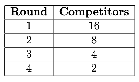
In 2024, the Olympics will include breaking (also known as breakdancing) for the first time. The breaking competition will include 16 athletes, who will compete in a single-elimination tournament.
In the first round, all 16 athletes will compete against an opponent in a face-to-face “battle". The 8 winners, as determined by the judges, will move on to the next round. Elimination continues until the final round contains just 2 competitors, and the winner of this final battle wins the tournament.
The table below shows how many competitors participate in each round:
After the 2024 Olympics, suppose we make a DataFrame called
breaking containing information about the performance of
each athlete during each round. breaking will have one row
for each athlete’s performance in each round that they participated.
Therefore, there will be 16+8+4+2 =
30 rows in breaking.
In the "name" column of breaking, we will
record the athlete’s name (which we’ll assume to be unique), and in the
other columns we’ll record the judges’ scores in the categories on which
the athletes will be judged (creativity, personality, technique,
variety, performativity, and musicality).
How many rows of breaking correspond to the winner of
the tournament? Give your answer as an integer.
Answer: 4
Since the winner of the tournament must have won during the 1st, 2nd,
3rd, and final rounds, there will be a total of four rows in
breaking corresponding to this winner.
The average score on this problem was 94%.
How many athletes’ names appear exactly twice in the
"name" column of breaking? Give your answer as
an integer.
Answer: 4
For an athlete to appear on exactly two rows in
breaking, they must get through the 1st round but get
eliminated in the 2nd round. There are a total of 8 athletes in the 2nd
round, of which 4 are eliminated.
The average score on this problem was 82%.
If we merge breaking with itself on the
"name" column, how many rows will the resulting DataFrame
have? Give your answer as an integer.
Hint: Parts (a) and (b) of this question are relevant to part (c).
Answer: 74
This question asks us the number of rows in the DataFrame that
results from merging breaking with itself on the name
column. Let’s break this problem down.
Concept:
When a DataFrame is merged with another DataFrame, there will be one row in the output DataFrame for every matching value between the two DataFrames in the row you’re merging on. In general, this means you can calculate the number of rows in the output DataFrame the following way:
\text{Number of instances of \texttt{a} in \texttt{df1} } \cdot \text{ Number of instances of \texttt{a} in \texttt{df2}} +
\text{Number of instances of \texttt{b} in \texttt{df1}} \cdot \text{Number of instances of \texttt{b} in \texttt{df2}} +
\vdots
\text{Number of instances of \texttt{n} in \texttt{df1}} \cdot \text{ Number of instances of \texttt{n} in \texttt{df2}}
For example, if there were 2
instances of "Jack" in df1 and 3 instances of "Jack" in
df2, there would be 2 \cdot 3 =
6 instances of "Jack" in the output DataFrame.
So, when we’re merging a DataFrame with itself, you can calculate the number of rows in the output DataFrame the following way:
\text{Number of instances of \texttt{a} in \texttt{df1} } \cdot \text{ Number of instances of \texttt{a} in \texttt{df1} } +
\text{Number of instances of \texttt{b} in \texttt{df1}} \cdot \text{Number of instances of \texttt{b} in \texttt{df1} } +
\vdots
\text{Number of instances of \texttt{n} in \texttt{df1}} \cdot \text{ Number of instances of \texttt{n} in \texttt{df1} }
which is the same as
\left(\text{Number of instances of \texttt{a} in \texttt{df1} }\right)^2
\left(\text{Number of instances of \texttt{b} in \texttt{df1} }\right)^2
\vdots
\left(\text{Number of instances of \texttt{n} in \texttt{df1} }\right)^2
The Problem:
So, if we can figure out how many instances of each athlete are in breaking, we can calculate the number of rows in the merged DataFrame by squaring these numbers and adding them together.
As it turns out, we can absolutely do this! Consider the following information, drawn from the DataFrame:
Using the formula above for calculating the number of rows in the output DataFrame when merging a DataFrame with itself:
For 8 athletes, they will appear 1^2 = 1 time in the merged DataFrame. For 4 athletes, they will appear 2^2 = 4 times in the merged DataFrame. For 2 athletes, they will appear 3^2 = 9 times in the merged DataFrame. And for the last 2 athletes, they will appear 4^2 = 16 times in the merged DataFrame.
So, the total number of rows in the merged DataFrame is
8(1) + 4(4) + 2(9) + 2(16) = 8 + 16 + 18 + 32 = 74 rows.
The average score on this problem was 39%.
Recall that the number of competitors in each round is 16, 8, 4, 2. Write one line of code that
evaluates to the array np.array([16, 8, 4, 2]). You
must use np.arange in your solution, and
you may not use np.array or the DataFrame
breaking.
Answer: 2 ** np.arange(4, 0, -1)
This problem asks us to write one line of code that evaluates to the
array np.array([16, 8, 4, 2]).
Concept:
Right away, it should jump out at you that these are powers of 2 in reverse order. Namely,
[2^4, 2^3, 2^2, 2^1].
The key insight is that exponentiation works element-wise on an array. In otherwords:
2 ** [4, 3, 2, 1] = [2^4, 2^3, 2^2, 2^1].
Given this information, it is simply a matter of constructing a call
to np.arange() that resuts in the array
[4, 3, 2, 1]. While there are many calls that achieve this
outcome, one example is with the call
np.arange(4, 0, -1).
So, the full expression that evaluates to
np.array([16, 8, 4, 2]) is
2 ** np.arange(4, 0, -1)
The average score on this problem was 38%.
We want to use the sample of data in olympians to
estimate the mean age of Olympic beach volleyball players.
Which of the following distributions must be normally distributed in order to use the Central Limit Theorem to estimate this parameter?
The age distribution of all Olympic athletes.
The age distribution of Olympic beach volleyball players.
The age distribution of Olympic beach volleyball in our sample.
None of the above.
Answer: None of the Above
The central limit theorem states that the distribution of possible sample means and sample sums is approximately normal, no matter the distribution of the population. Options A, B, and C are not probability distributions of the sum or mean of a large random sample draw with replacement.
The average score on this problem was 72%.
(10 pts) Next we want to use bootstrapping to estimate this
parameter. Which of the following code implementations correctly
generates an array called sample_means containing 10,000 bootstrapped sample means?
Way 1:
    sample_means = np.array([])
    for i in np.arange(10000):
        bv = olympians[olympians.get("Sport") == "Beach Volleyball"]
        one_mean = (bv.sample(bv.shape[0], replace=True)
                      .get("Age").mean())
        sample_means = np.append(sample_means, one_mean)
Way 2:
    sample_means = np.array([])
    for i in np.arange(10000):
        bv = olympians[olympians.get("Sport") == "Beach Volleyball"]
        one_mean = (olympians.sample(olympians.shape[0], replace=True)
                             .get("Age").mean())
        sample_means = np.append(sample_means, one_mean)
Way 3:
    sample_means = np.array([])
    for i in np.arange(10000):
        resample = olympians.sample(olympians.shape[0], replace=True)
        bv = resample[resample.get("Sport") == "Beach Volleyball"]
        one_mean = bv.get("Age").mean()
        sample_means = np.append(sample_means, one_mean)
Way 4:
    sample_means = np.array([])
    bv = olympians[olympians.get("Sport") == "Beach Volleyball"]
    for i in np.arange(10000):
        one_mean = (bv.sample(bv.shape[0], replace=True)
                      .get("Age").mean())
        sample_means = np.append(sample_means, one_mean)
Way 5:
    sample_means = np.array([])
    bv = olympians[olympians.get("Sport") == "Beach Volleyball"]
    one_mean = (bv.sample(bv.shape[0], replace=True)
                  .get("Age").mean())
    for i in np.arange(10000):
        sample_means = np.append(sample_means, one_mean)
Way 1
Way 2
Way 3
Way 4
Way 5
Answer: Way 1 and Way 4
bv, which is a subset
DataFrame of olympians but filtered to only have
"Beach Volleyball". It then samples from bv
with replacement, and counts the mean of that sample and stores it in
the variable one_sample. It does this 10,000 times (due to
the for loop), each time creating a dataframe bv, sampling
from it, calculating a mean, and then appending one_sample
to the array sample_means. This is a correct way to
bootstrap.olympians DataFrame, instead of the bv
DataFrame with only the "Beach Volleyball" players. This
will result in a sample of players of any sport, and the mean of those
ages will be calculated."Sport" column equals "Beach Volleyball" after
sampling from the DataFrame instead of before. This would lead to a mean
that is not representative of a sample of volleyball players’ ages
because we are sampling from all the rows with all different sports,
most likely resulting in a smaller sample size of volleyball players.
There would also be an inconsistent number of
"Beach Volleyball" players in each sample.bv before the for loop. The DataFrame
bv will always be the same, so it doesn’t really matter if
we make bv before or after the for loop.one_mean is calculated
only once, but is appended to the sample_means array 10,000
times. As a result, the same mean is being appended, instead of a
different mean being calculated and appended each iteration.
The average score on this problem was 88%.
For most of the answer choices in part (b), we do not have enough
information to predict how the standard deviation of
sample_means would come out. There is one answer choice,
however, where we do have enough information to compute the standard
deviation of sample_means. Which answer choice is this, and
what is the standard deviation of sample_means for this
answer choice?
Way 1
Way 2
Way 3
Way 4
Way 5
Answer: Way 5
Way 5 results in a sample_means array with the same mean appended 10,000 times. As a result the standard deviation would be 0 because the entire array would be the same value repeated.
The average score on this problem was 57%.
There are 68 rows of olympians
corresponding to beach volleyball players. Assume that in part (b), we
correctly generated an array called sample_means containing
10,000 bootstrapped sample mean ages based on this original sample of 68
ages. The standard deviation of the original sample of 68 ages is
approximately how many times larger than the standard deviation of
sample_means? Give your answer to the nearest integer.
Answer: 8
Recall SD of sample_means = \frac{\text{Population SD}}{\sqrt{\text{sample size}}}. The sample size equals 68. Based on this equation, the population SD is \sqrt{68} times larger than the SD of distribution of possible sample means. \sqrt{68} rounded to the nearest integer is 8.
The average score on this problem was 46%.
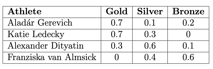
Aladár Gerevich is a Hungarian fencer who is one of only two men to win Olympic medals 28 years apart. He earned 10 Olympic medals in total throughout his career: 7 gold, 1 silver, and 2 bronze. The table below shows the distribution of medal types for Aladár Gerevich, as well as a few other athletes who also earned 10 Olympic medals.
Which type of data visualization is most appropriate to compare two athlete’s medal distributions?
overlaid histogram
overlaid bar chart
overlaid line plot
Answer: overlaid bar chart
Here, we are plotting the data of 2 athletes, comparing the medal distributions. Gold, silver, and bronze medals are categorical variables, while the proportion of these won is a quantitative value. A bar chart is the only kind of plot that involves categorical data with quantitative data. Since there are 2 athletes, the most appropriate plot is an overlaid bar chart. The overlapping bars would help compare the difference in their distributions.
The average score on this problem was 73%.
Among the other athletes in the table above, whose medal distribution has the largest total variation distance (TVD) to Aladár Gerevich’s distribution?
Katie Ledecky
Alexander Dityatin
Franziska van Almsick
Answer: Franziska van Almsick
The Total Variation Distance (TVD) of two categorical distributions is the sum of the absolute differences of their proportions, all divided by 2. We can apply the TVD formula to these distributions: The TVD between Katie Ledecky and Aladar Gerevich is given by \frac{1}{2} \cdot (|0.7 - 0.7| + |0.1 - 0.3| + |0.2 - 0|) = \frac{0.4}{2} = 0.2. The TVD between Alexander Dityatin and Aladar Gerevich is given by \frac{1}{2} \cdot (|0.7 - 0.3| + |0.1 - 0.6| + |0.2 - 0.1|) = \frac{1}{2} = 0.5. And finally, the TVD between Franziska van Almsick and Aladar Gerevich is given by \frac{1}{2} \cdot (|0.7 - 0| + |0.1 - 0.4| + |0.2 - 0.6|) = \frac{1.4}{2} = 0.7. So, Franziska van Almsick has the largest TVD to Gerevich’s distribution.
The average score on this problem was 92%.
Suppose Pallavi earns 10 Olympic medals in such a way that the TVD between Pallavi’s medal distribution and Aladár Gerevich’s medal distribution is as large as possible. What is Pallavi’s medal distribution?
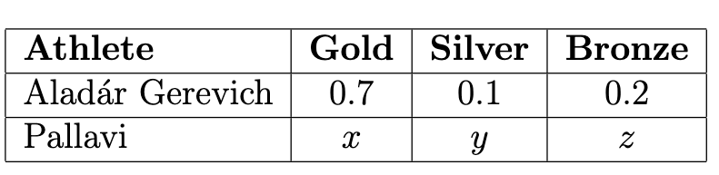
Answer: x=0, y=1, z=0
Intuitively, can maximize the TVD between the distributions by putting all of Pallavi’s medals in the category which Gerevich won the least of, so x = 0, y = 1, z = 0. Moving any of these medals to another category would decrease the TVD, since that would mean that all of Pallavi’s medal proportions would get closer to Gerevich’s (Silver is decreasing, getting closer, and Gold and Bronze are increasing, which makes them closer as well).
The average score on this problem was 72%.
More generally, suppose medal_dist is an array of length
three representing an athlete’s medal distribution. Which of the
following expressions gives the maximum possible TVD between
medal_dist and any other distribution?
medal_dist.max()
medal_dist.min()
1 - medal_dist.max()
1 - medal_dist.min()
np.abs(1 - medal_dist).sum()/2
Answer: 1 - medal_dist.min()
Similar to part c, we know that the TVD is maximized by placing all
the medals of competitor A into the category in which competitor B has
the lowest proportion of medals. If we place all of competitor A’s
medals into this bin, the difference between the two distributions for
this variable will be 1 - medal_dist.min() In the other
bins, competitor A has no medals (making all their values 0), and
competitor B has the remainder of their medals, which is
1 - medal_dist.min(). So, in total, the TVD is given by
\frac{1}{2} \cdot 2 \cdot
1 - medal_dist.min() =
1 - medal_dist.min().
The average score on this problem was 56%.
Consider the DataFrame
olympians.drop(columns=["Medal", "Year", "Count"]).
State a question we could answer using the data in this DataFrame and a permutation test.
Answer: There are many possible answers for this question. Some examples: “Are male olympians from Team USA significantly taller than male olympians from other countries?”, “Are olympic swimmers heavier than olympic figure skaters?”, “On average, are male athletes heavier than female athletes?” Any question asking for a difference in a numerical variable across olympians from different categories would work, as long as it is not about the dropped columns.
Recall that a permutation test is basically trying to test if two variables come from the same distribution or if the difference between those two variables are so significant that we can’t possibly say that they’re from the same distribution. In general, this means the question would have to involve the age, height, or weight column because they are numerical data.
The average score on this problem was 80%.
State the null and alternative hypotheses for this permutation test.
Answer: Also many possible answers depending on your answer for the first question.
For example, if our question was “Are olympic swimmers heavier than olympic figure skaters?”, then the null hypothesis could be “Olympic swimmers weigh the same as olympic figure skaters” and the alternative could be “Olympic swimmers weigh more than figure skaters.”
The average score on this problem was 80%.
In our sample, we have data on 163 medals for the sport of table tennis. Based on our data, China seems to really dominate this sport, earning 81 of these medals.
That’s nearly half of the medals for just one country! We want to do a hypothesis test with the following hypotheses to see if this pattern is true in general, or just happens to be true in our sample.
Null: China wins half of Olympic table tennis medals.
Alternative: China does not win half of Olympic table tennis medals.
Why can these hypotheses be tested by constructing a confidence interval?
Since proportions are means, so we can use the CLT.
Since the test aims to determine whether a parameter is equal to a fixed value.
Since we need to get a sense of how other samples would come out by bootstrapping.
Since the test aims to determine if our sample came from a known population distribution.
Answer: Since the test aims to determine whether a parameter is equal to a fixed value
The goal of a confidence interval is to provide a range of values that, given the data, are considered plausible for the parameter in question. If the null hypothesis’ fixed value does not fall within this interval, it suggests that the observed data is not very compatible with the null hypothesis. Thus in our case, if a 95% confidence interval for the proportion of medals won by China does not include ~0.5, then there’s statistical evidence at the 5% significance level to suggest that China does not win exactly half of the medals. So again in our case, confidence intervals work to test this hypothesis because we are attempting to find out whether or half of the medals (0.5) lies within our interval at the 95% confidence level.
The average score on this problem was 44%.
Suppose we construct a 95% bootstrapped CI for the proportion of Olympic table tennis medals won by China. Select all true statements.
The true proportion of Olympic table tennis medals won by China has a 95% chance of falling within the bounds of our interval.
If we resampled our original sample and calculated the proportion of Olympic table tennis medals won by China in our resample, there is approximately a 95% chance our interval would contain this number.
95% of Olympic table tennis medals are won by China.
None of the above.
Answer: If we resampled our original sample and calculated the proportion of Olympic table tennis medals won by China in our resample, there is approximately a 95% chance our interval would contain this number.
The second option is the only correct answer because it accurately describes the process and interpretation of a bootstrap confidence interval. A 95% bootstrapped confidence interval means that if we repeatedly sampled from our original sample and constructed the interval each time, approximately 95% of those intervals would contain the true parameter. This statement does not imply that the true proportion has a 95% chance of falling within any single interval we construct; instead, it reflects the long-run proportion of such intervals that would contain the true proportion if we could repeat the process indefinitely. Thus, the confidence interval gives us a method to estimate the parameter with a specified level of confidence based on the resampling procedure.
The average score on this problem was 73%.
True or False: In this scenario, it would also be appropriate to create a 95% CLT-based confidence interval.
True
False
Answer: True
The statement is true because the Central Limit Theorem (CLT) applies to the sampling distribution of the proportion, given that the sample size is large enough, which in our case, with 163 medals, it is. The CLT asserts that the distribution of the sample mean (or proportion, in our case) will approximate a normal distribution as the sample size grows, allowing the use of standard methods to create confidence intervals. Therefore, a CLT-based confidence interval is appropriate for estimating the true proportion of Olympic table tennis medals won by China.
The average score on this problem was 71%.
True or False: If our 95% bootstrapped CI came out to be [0.479, 0.518], we would reject the null hypothesis at the 0.05 significance level.
True
False
Answer: False
This is false, we would fail to reject the null hypothesis because the interval [0.479, 0.518] includes the value of 0.5, which corresponds to the null hypothesis that China wins half of the Olympic table tennis medals. If the confidence interval contains the hypothesized value, there is not enough statistical evidence to reject the null hypothesis at the specified significance level. In this case, the data does not provide sufficient evidence to conclude that the proportion of medals won by China is different from 0.5 at the 0.05 significance level.
The average score on this problem was 92%.
True or False: If we instead chose to test these hypotheses at the 0.01 significance level, the confidence interval we’d create would be wider.
True
False
Answer: True
Lowering the significance level means that you require more evidence to reject the null hypothesis, thus seeking a higher confidence in your interval estimate. A higher confidence level corresponds to a wider interval because it must encompass a larger range of values to ensure that it contains the true population parameter with the increased probability. Thus as we lower the significance level, the interval we create will be wider, making this statement true.
The average score on this problem was 79%.
True or False: If we instead chose to test these hypotheses at the 0.01 significance level, we would be more likely to conclude a statistically significant result.
True
False
Answer: False
This statement is false. A small significance level lowers the chance of getting a statistically significant result; our value for 0.01 significance has to be outside a 99% confidence interval to be statistically significant. In addition, the true parameter was already contained within the tighter 95% confidence interval, so we failed to reject the null hypothesis at the 0.05 significance level. This guarantees failing to reject the null hypotehsis at the 0.01 significance level since we know that whatever is contained in a 95% confidence interval has to also be contained in a 99% confidence interval. Thus, this answer is false.
The average score on this problem was 62%.
Suppose that in Olympic ski jumping, ski jumpers jump off of a ramp that’s shaped like a portion of a normal curve. Drawn from left to right, a full normal curve has an inflection point on the ascent, then a peak, then another inflection point on the descent. A ski jump ramp stops at the point that is one third of the way between the inflection point on the ascent and the peak, measured horizontally. Below is an example ski jump ramp, along with the normal curve that generated it.
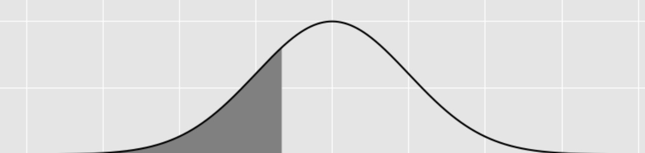
Fill in the blank below so that the expression evaluates to the area of a ski jump ramp, if the area under the normal curve that generated it is 1.
    from scipy import stats
    stats.norm.cdf(______)
What goes in the blank?
Answer: -2/3
We know that the normal distribution is symmetric about the mean, and
that the mean is the “peak” described in the graph. The inflection
points occur one standard deviation above and below the mean (the peak),
so a point which is one third of the way in between the first inflection
point and the peak is -(1-\frac{1}{3}) =
-\frac{2}{3} standard deviations from the mean. We can then use
stats.norm.cdf(-2/3) to calculate the area under the curve
to the left of this point.
The average score on this problem was 51%.
Suppose that in Olympic downhill skiing, skiers compete on mountains shaped like normal distributions with mean 50 and standard deviation 8. Skiers start at the peak and ski down the right side of the mountain, so their x-coordinate increases.
Keenan is an Olympic downhill skier, but he’s only been able to practice on a mountain shaped like a normal distribution with mean 65 and standard deviation 12. In his practice, Keenan always crouches down low when he reaches the point where his x-coordinate is 92, which helps him ski faster. When he competes at the Olympics, at what x-coordinate should he crouch down low, corresponding to the same relative location on the mountain?
Answer: 68
Since we know that both slopes are normal distributions (just scaled and shifted), we can derive this answer by writing Keenan’s crouch point in terms of standard deviations from the mean. He typically crouches at 92 feet, whose distance from the mean (in standard deviations) is given by \frac{92 - 65}{12} = 2.25. So, all we need to do is find what number is 2.25 standard deviations from the mean in the Olympic mountain. This is given by 50 + (2.25 * 8) = 68
The average score on this problem was 72%.
Aaron is another Olympic downhill skier. When he competes on the normal curve mountain with mean 50 and standard deviation 8, he crouches down low when his x-coordinate is 54. If the total area of the mountain is 1, approximately how much of the mountain’s area is ahead of Aaron at the moment he crouches down low?
0.1
0.2
0.3
0.4
Answer: 0.3
We know that when Aaron reaches the mean (50), exactly 0.5 of the mountain’s area is behind him, since the mean and median are equal for normal distributions like this one. We also see that 54 is one half of a standard deviation away from the mean. So, all we have to do is find out what proportion of the area is within half a standard deviation of the mean. Using the 68-95-99.7 rule, we know that 68% of the values lie within one standard deviation of the mean to both the right and left side. So, this means 34% of the values are within one standard deviation on one side and at least 17% are within half a standard deviation on one side. Since the area is 1, the area would be 0.17. So, by the time Aaron reaches an x-coordinate of 54, 0.5 + 0.17 = 0.67 of the mountain is behind him. From here, we simply calculate the area in front by 1 - 0.67 = 0.33, so we conclude that approximately 0.3 of the area is in front of Aaron.
Note: As a clafrification, the 0.17 is an estimate, specifically, an underestimate, due to the shape of the normal distribution. Thse area under a normal distribution is not proportional to how many standard deviations far away from the mean you are.
The average score on this problem was 50%.
Birgit Fischer-Schmidt is a German canoe paddler who set many records, including being the only woman to win Olympic medals 24 years apart.
Below is a DataFrame with information about all 12 Olympic medals she has won. There are only 10 rows but 12 medals represented, because there are some years in which she won more than one medal of the same type.
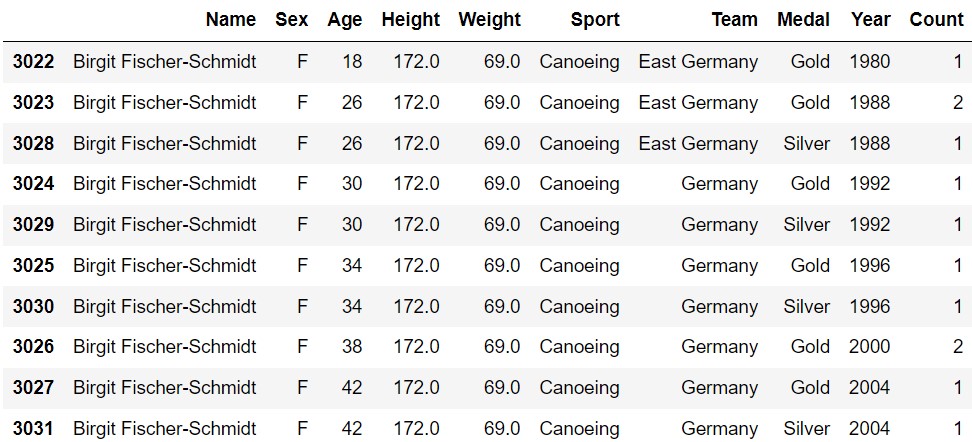
Suppose we randomly select one of Birgit’s Olympic medals, and see that it is a gold medal. What is the probability that the medal was earned in the year 2000? Give your answer as a fully simplified fraction.
Answer: \frac{1}{4}
Reading the prompt we can see that we are solving for a conditional probability. Let A be the given condition that the medal is gold and let B be the event that a medal is from 2000. Looking at the DataFrame we can see that 8 total gold medals are earned (make sure you pay attention to the count column). Out of these 8 medals, 2 of them are from the year 2000. Thus, we obtain the probability \frac{2}{8} or \frac{1}{4}.
The average score on this problem was 70%.
Suppose we randomly select one of Birgit’s Olympic medals. What is the probability it is gold or earned while representing East Germany? Give your answer as a fully simplified fraction.
Answer: \frac{3}{4}
Here we can recognize that we are solving for the probability of a union of two events. Let A be the event that the medal is gold. Let B be the event that it is earned while representing East Germany. The probability formula for a union is P(A \cup B) = P(A) + P(B) - P(A \cap B). Looking at the DataFrame, we know P(A)=\frac{8}{12}, P(B)=\frac{4}{12}, and P(A \cap B)=\frac{3}{12}. Plugging all of this into the formula, we get \frac{8}{12}+\frac{4}{12}-\frac{3}{12}=\frac{9}{12}=\frac{3}{4}. Thus, the correct answer is \frac{3}{4}.
The average score on this problem was 73%.
Suppose we randomly select two of Birgit’s Olympic medals, without replacement. What is the probability both were earned in 1988? Give your answer as a fully simplified fraction.
Answer: \frac{1}{22}
In this problem, we are sampling 2 medals without replacement. Let A be the event that the first medal is from 1988 and let P(B) be the event that the second medal is from 1988. P(A) is \frac{3}{12} since there are 3 medals from 1988 out of the total 12 medals. However, in the second trial, since we are sampling without replacement, the medal that we just sampled is no longer in our pool. Thus, P(B) is now \frac{2}{11} since there are now 2 medals from 1988 from the remaining 11 total medals. The joint probability P(A \cap B) is P(A)P(B) so, plugging these values in, we get \frac{3}{12} \cdot \frac{2}{11} = \frac{3}{66} = \frac{1}{22}. Thus, the answer is \frac{1}{22}.
The average score on this problem was 57%.
Suppose males is a DataFrame of all male Olympic
weightlifting medalists with a column called "Weight"
containing their body weight. Similarly, females is a
DataFrame of all female Olympic weightlifting medalists. It also has a
"Weight" column with body weights.
The males DataFrame has 425 rows and
the females DataFrame has 105 rows, since
women’s weightlifting became an Olympic sport much later than men’s.
Below, density histograms of the distributions of
"Weight" in males and females are
shown on the same axes:
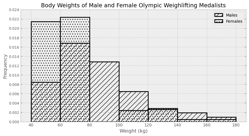
Estimate the number of males included in the third bin (from 80 to 100). Give your answer as an integer, rounded to the nearest multiple of 10.
Answer: 110
We can estimate the number of males included in the third bin (from 80 to 100) by multiplying the area of that particular histogram bar by the total number of males. The bar has a height of around 0.013 and a width of 20, so the bar has an area of 0.013 \cdot 20 = 0.26, which means 26% of males fall in that bin. Since there are 425 total males, 0.26 \cdot 425 ≈ 110 males are in that bin, rounded to the nearest multiple of 10.
The average score on this problem was 81%.
Using the males DataFrame, write one line of code that
evaluates to the exact number of males included in the third bin (from
80 to 100).
Answer:
males[(males.get("Weight")>=80) & (males.get("Weight")<100)].shape[0]
To get the exact number of males in the third bin (from 80 to 100)
using code, we can query the males DataFrame to only include rows where
"Weight" is greater than or equal to 80, and
"Weight" is less than 100. Remember, a histogram bin
includes the lower bound (in this case, 80) and excludes the upper bound
(in this case, 100). Remember to put parentheses around each condition,
or else the order of operations will change your intended conditions.
After querying, we use .shape[0] to get the number of rows
in that dataframe, therefore getting the number of males with a weight
greater than or equal to 80, and less than 100.
The average score on this problem was 75%.
Among Olympic weightlifting medalists who weigh less than 60 kilograms, what proportion are male?
less than 0.25
between 0.25 and 0.5
between 0.5 and 0.75
more than 0.75
Answer: between 0.5 and 0.75
We can answer this question by calculating the approximate number of males and females in the first bin (from 40 to 60). Be careful, we cannot simply compare the areas of the bars because the number of male weightlifting medalists is different from the number of female weightlifting medalists. The approximate number of male weightlifting medalists is equal to 0.008 \cdot 20 \cdot 425 = 68, while the approximate number of female weightlifting medalists is equal to 0.021 \cdot 20 \cdot 105 = 44. The proportion of male weightlifting medalists who weigh less than 69 kg is approximately \frac{68}{68 + 44} = 0.607, which falls in the category of “between 0.5 and 0.75”.
The average score on this problem was 54%.