← return to practice.dsc10.com
Instructor(s): Janine Tiefenbruck
This exam was administered in-person. Students were allowed one page of double-sided handwritten notes. No calculators were allowed. Students had 3 hours to take this exam.
Note (groupby / pandas 2.0): Pandas 2.0+ no longer
silently drops columns that can’t be aggregated after a
groupby, so code written for older pandas may behave
differently or raise errors. In these practice materials we use
.get() to select the column(s) we want after
.groupby(...).mean() (or other aggregations) so that our
solutions run on current pandas. On real exams you will not be penalized
for omitting .get() when the old behavior would have
produced the same answer.
While browsing the library, Hermione stumbles upon an old book containing game logs for all Quidditch matches played at Hogwarts in the 18th century. Quidditch is a sport played between two houses. It features three types of balls:
Quaffle: Worth 10 points when used to score a goal.
Bludger: Does not contribute points. Instead, used to distract the other team.
Snitch: Worth 150 points when caught. This immediately ends the game.
A game log is a list of actions that occurred during a Quidditch
match. Each element of a game log is a two-letter string where the first
letter represents the house that performed the action ("G"
for Gryffindor, , "H" for Hufflepuff, "R" for
Ravenclaw, "S" for Slytherin) and the second letter
indicates the type of Quidditch ball used in the action
("Q" for Quaffle, "B" for Bludger,
"S" for Snitch). For example, "RQ" in a game
log represents Ravenclaw scoring with the Quaffle to earn 10 points.
Hermione writes a function, logwarts, to calculate the
final score of a Quidditch match based on the actions in the game log.
The inputs are a game log (a list, as described above) and the full
names of the two houses competing. The output is a list of length 4
containing the names of the teams and their corresponding scores.
Example behavior is given below.
    >>> logwarts(["RQ", "GQ", "RB", "GS"], "Gryffindor", "Ravenclaw")
    ["Gryffindor", 160, "Ravenclaw", 10]

    >>> logwarts(["HB", "HQ", "HQ", "SS"], "Hufflepuff", "Slytherin")
    ["Hufflepuff", 20, "Slytherin", 150]
Fill in the blanks in the logwarts function below. Note
that some of your answers are used in more than one
place in the code.
    def logwarts(game_log, team1, team2):
        score1 = __(a)__
        score2 = __(a)__

        for action in game_log:
            house = __(b)__
            ball = __(c)__

            if __(d)__:
                __(e)__:
                    score1 = score1 + 10
                __(f)__:
                    score1 = score1 + 150
            else:
                __(e)__:
                    score2 = score2 + 10
                __(f)__:
                    score2 = score2 + 150
return [team1, score1, team2, score2]What goes in blank (a)?
Answer: 0
First inspect the function parameters. With the example
logwarts(["RQ", "GQ", "RB", "GS"], "Gryffindor", "Ravenclaw"),
we observe game_log will be a list of strings, and
team1 and team2 will be the full name of the
respective competing houses. We can infer from the given structure that
our code will
Initialize two scores variables for the two houses,
Run a for loop through all the entries in the list, update score based on given conditions,
Return the scores calculated by the loop.
To set up score_1 and score_2 so we can
accumulate them in the for loop, we first set both equal to 0. So blank
(a) will be 0.
The average score on this problem was 89%.
What goes in blank (b)?
Answer: action[0]
We observe the for loop iterates over the list of actions, where each
action is a two letter string in the
game_log array. Recall question statement- “Each element of
a game log is a two-letter string where the first letter represents the
house that performed the action”. Therefore, to get the house, we will
want to get the first letter of each action string. This is accessed by
action[0].
Note: A common mistake here is using action.split()[0].
Recall
what split() does - it takes in a string, splits it
according to the delimiter given (if not given, it separates by blank
space), and returns a list of separated strings. This
means that action.split()[0] will actually return itself.
Example: if action is "RQ",
action.split() will split "RQ" by blank space,
in this case, there are none; so it will return the one-element list
["RQ"]. Accessing the zero-th index of this list by
action.split()[0] gives us "RQ" back, instead
of what we actually want ("R").
The average score on this problem was 61%.
What goes in blank (c)?
Answer: action[1]
Following the same logic as blank (b), we get the type of ball used
in the action by accessing the second character of the string, which is
action[1].
The average score on this problem was 62%.
What goes in blank (d)?
Answer: house == team1[0]
Now enter the fun part: to figure out the correct conditions of the if-statments, we must observe the code inside our conditional blocks carefully.
Recall question statement:
For each entry of the game log, the house is represented by the first letter. “G” for Griffindor, “H” for Hufflepuff, “R” for Ravenclaw, “S” for Slytherin.
Quaffle (“Q”) gets 10 points,
Snitch (“S”) gets 150 points,
Bludger (“B”) gets no point.
score1 is the score of the first team, and
score2 is the score of the second.
We have two conditions to take care of, the house and the type of
ball. How on earth do we know which one is nested and which one is on
the outside? Observe in the first big if statment, we are only updating
score1. This means this block takes care of the score of
the first house. Therefore, blank (d) should set the condition for the
first house.
Now careful! team1 and team2 are given as
full house names. We can match the house variable by
getting the first letter of the each team string (e.g. if
team1 is Griffindor, we will get “G” to match with “G”). We
want to match house with team1[0], so our
final answer is house == team1[0]. Since there are only two
houses here, the following else block will take care of
calculating score for the second house using the same scoring scheme as
we do for the first house.
The average score on this problem was 74%.
What goes in blank (e)?
Answer: if ball == "Q"
After gracefully handling the outer conditional statement, the rest
is simple. We now simply condition the scores. Here, we see score1
increments by 10, so we know this is accounting for a Quaffle. Recall
ball variable represents the type of ball we have. In this
case, we use if ball == "Q" to filter for Quaffles.
The average score on this problem was 69%.
What goes in blank (f)?
Answer: elif ball == "S" or
if ball == "S"
Using the same logic as blank (e), since the score is incremented by
150 here, we know this is a snitch. Using elif ball == "S"
or if ball == "S" will serve the purpose. We do not need to
worry about bludgers, since those do not add to the score.
The average score on this problem was 64%.
The Death Eaters are a powerful group of dark wizards who oppose
Harry Potter and his allies. Each Death Eater receives a unique
identification number based on their order of initiation, ranging from
1 to N, where N represents the
total number of Death Eaters.
Your task is to estimate the value of N so you can
understand how many enemies you face. You have a random sample of
identification numbers in a DataFrame named death_eaters
containing a single column called "ID".
Which of the options below would be an appropriate estimate for the total number of Death Eaters? Select all that apply.
death_eaters.get("ID").max()
death_eaters.get("ID").sum()
death_eaters.groupby("ID").count()
int(death_eaters.get("ID").mean() * 2)
death_eaters.shape[0]
None of the above.
Answer: death_eaters.get("ID").max()
and int(death_eaters.get("ID").mean() * 2)
Option 1: death_eaters.get("ID").max() returns the
maximum ID from the sample. This is an appropriate estimate since the
population size must be at least the size of the largest ID in our
sample. For instance, if the maximum ID observed is 250, then the total
number of Death Eaters must be at least 250.
Option 2: death_eaters.get("ID").sum() returns the
sum of all ID numbers in the sample. The total sum of IDs has no
meaningful connection to the population size, which makes this an
inappropriate estimate.
Option 3: death_eaters.groupby("ID").count() groups
the data by ID and counts occurrences. Since each ID is unique and
death_eaters only includes the "ID" column,
grouping simply shows that each ID appears once. This is not an
appropriate estimate for N.
Option 4: int(death_eaters.get("ID").mean() * 2)
returns twice the mean of the sample IDs as an integer. The mean of a
random sample of the numbers 1 through N usually falls
about halfway between 1 and N. So we can appropriately
estimate N by doubling this mean.
Option 5: death_eaters.shape[0] returns the number
of rows in death_eaters (ie. the sample size). The sample
size does not reflect the total population size, making it an
inappropriate estimate.
The average score on this problem was 66%.
Each box that you selected in part (a) is an example of what?
a distribution
a statistic
a parameter
a resample
Answer: a statistic
The options in part (a) calculate a numerical value from the random
sample death_eaters. This fits the definition of a
statistic.
The average score on this problem was 82%.
Suppose you have access to a function called estimate,
which takes in a Series of Death Eater ID numbers and returns an
estimate for N. Fill in the blanks below to do the
following:
Create an array named boot_estimates, containing
10,000 of these bootstrapped estimates of N, based on the
data in death_eaters.
Set left_72 to the left endpoint of
a 72% confidence interval for N.
    boot_estimates = np.array([])

    for i in np.arange(10000):
        boot_estimates = np.append(boot_estimates, __(a)__)

    left_72 = __(b)__
What goes in blank (a)?
Answer:
estimate(death_eaters.sample(death_eaters.shape[0], replace=True).get("ID"))
In the given code, we use a for loop to generate 10,000 bootstrapped
estimates of N and append them to the array
boot_estimates. Blank (a) specifically computes one
bootstrapped estimate of N. Here’s how key parts of the
solution work:
death_eaters.sample(death_eaters.shape[0], replace=True):
To bootstrap, we need to resample the data with replacement. The
sample() function
(see
here) takes as arguments the sample size
(death_eaters.shape[0]) and whether to replace
(replace=True).
.get("ID"): Since estimate() takes a
Series as input, we need to extract the ID column from the
resample.
estimate(): The resampled ID column is passed into
the estimate() function to generate one bootstrapped
estimate of N.
The average score on this problem was 62%.
What goes in blank (b)?
Answer:
np.percentile(boot_estimates, 14)
A 72% confidence interval captures the middle 72% of our
distribution. This leaves 28% of the data outside the interval, with 14%
from the lower tail and 14% from the upper tail. Thus, the left endpoint
corresponds to the 14th percentile of boot_estimates. The
np.percentile() function
(see
here) takes as arguments the array to compute the percentile
(boot_estimates) and the desired percentile (14).
The average score on this problem was 91%.
When new students arrive at Hogwarts, they get assigned to one of the four houses (Gryffindor, Hufflepuff, Ravenclaw, Slytherin) by a magical Sorting Hat.
Throughout this problem, we’ll assume that the Sorting Hat assigns students to houses uniformly at random, meaning that each student has an independent 25% chance of winding up in each of the four houses.
For all parts, give your answer as an unsimplified mathematical expression.
There are seven siblings in the Weasley family: Bill, Charlie, Percy, Fred, George, Ron, and Ginny. What is the probability that all seven of them are assigned to Gryffindor?
Answer: \left(0.25\right)^{7}
The probability that a student gets assigned to Gryffindor is 0.25 (or \frac{1}{4}). Since we are given that the Sorting Hat assigns students independently, we can apply the multiplication rule and multiply the probability of each of the seven Weasleys being sorted to Gryffindor together. Therefore, all terms in our product are 0.25. Thus, the probability that all seven Weasleys get assigned to Gryffindor would be 0.25 * 0.25 * \ldots * 0.25 = \left(0.25\right)^{7}.
The average score on this problem was 94%.
What is the probability that Fred and George Weasley are assigned to the same house?
Answer: 0.25
Fred and George are assigned to the same house if both are in Gryffindor, or both are in Hufflepuff, etc.. Fred and George’s selections from the sorting hat are independent. Using the multiplication rule, P(both in Gryffindor) = 0.25 * 0.25. Likewise, P(both in Hufflepuff) = 0.25 * 0.25. It is the same for Ravenclaw and Slytherin as well. Therefore, P(same house) = 4 * (0.25 * 0.25) = 0.25.
The average score on this problem was 68%.
What is the probability that none of the seven Weasley siblings are assigned to Slytherin?
Answer: \left(0.75\right)^{7}
The probability that none of the seven Weasley siblings are assigned to Slytherin is equal to the probability that all of the Weasley siblings are not assigned to Slytherin. The probability that someone is not assigned to Slytherin is 1 - P(Slytherin) = 1 - 0.25 = 0.75. Since we are given that the Sorting Hat assigns students independently, we can apply the multiplication rule and multiply the probability of each of the seven Weasleys being sorted to anywhere but Slytherin together. Therefore, all terms in our product are 0.75. Thus, the probability that none of seven Weasleys get assigned to Slytherin would be 0.75 * 0.75 * \ldots * 0.75 = \left(0.75\right)^{7}.
The average score on this problem was 67%.
Suppose you are told that none of the seven Weasley siblings are assigned to Slytherin. Based on this information, what is the probability that at least one of the siblings is assigned to Gryffindor?
Answer: 1 - \left(\frac{2}{3}\right)^{7}
Since we are given that none of the Weasley siblings are assigned to Slytherin, our possibilities are now only Gryffindor, Hufflepuff, and Ravenclaw. Therefore, the probability that someone is assigned to Gryffindor would become \frac{1}{3}. Correspondingly, the probability that someone isn’t assigned to Gryffindor is 1 - \frac{1}{3} = \frac{2}{3}. The probability that at least one of the siblings is assigned to Gryffindor is equal to 1 - the probability that none of the siblings are assigned to Gryffindor, or 1 - \left(\frac{2}{3}\right)^{7}.
The average score on this problem was 51%.

Beneath Gringotts Wizarding Bank, enchanted mine carts transport wizards through a complex underground railway on the way to their bank vault.
During one section of the journey to Harry’s vault, the track follows the shape of a normal curve, with a peak at x = 50 and a standard deviation of 20.
A ferocious dragon, who lives under this section of the railway, is equally likely to be located anywhere within this region. What is the probability that the dragon is located in a position with x \leq 10 or x \geq 80? Select all that apply.
1 - (scipy.stats.norm.cdf(1.5) - scipy.stats.norm.cdf(-2))
2 * scipy.stats.norm.cdf(1.75)
scipy.stats.norm.cdf(-2) + scipy.stats.norm.cdf(-1.5)
0.95
None of the above.
Answer:
1 - (scipy.stats.norm.cdf(1.5) - scipy.stats.norm.cdf(-2))
&
scipy.stats.norm.cdf(-2) + scipy.stats.norm.cdf(-1.5)
Option 1: This code calculates the probability that a value lies outside the range between z = -2 and z = 1.5, which corresponds to x \leq 10 or x \geq 80. This is done by subtracting the area under the normal curve between -2 and 1.5 from 1. This is correct because it accurately captures the combined probability in the left and right tails of the distribution.
Option 2: This code multiplies the cumulative distribution function (CDF) at z = 1.75 by 2. This assumes symmetry around the mean and is used for intervals like |z| \geq 1.75, but that’s not what we want. The correct z-values for this problem are -2 and 1.5, so this option is incorrect.
Option 3: This code adds the probability of z \leq -2 and z \geq 1.5, using the fact that P(z \geq 1.5) = P(z \leq -1.5) by symmetry. So, while the code appears to show both as left-tail calculations, it actually produces the correct total tail probability. This option is correct.
Option 4: This is a static value with no basis in the z-scores of -2 and 1.5. It’s likely meant as a distractor and does not represent the correct probability for the specified conditions. This option is incorrect.
Harry wants to know where, in this section of the track, the cart’s height is changing the fastest. He knows from his earlier public school education that the height changes the fastest at the inflection points of a normal distribution. Where are the inflection points in this section of the track?
x = 50
x = 20 and x = 80
x = 30 and x = 70
x = 0 and x = 100
Answer: x = 30 and x = 70
Recall that the inflection points of a normal distribution are located one standard deviation away from the mean. In this problem, the mean is x = 50 and the standard deviation is 20, so the inflection points occur at x = 30 and x = 70. These are the points where the curve changes concavity and where the height is changing the fastest. Therefore, the correct answer is x = 30 and x = 70.
Next, consider a different region of the track, where the shape follows some arbitrary distribution with mean 130 and standard deviation 30. We don’t have any information about the shape of the distribution, so it is not necessarily normal.
What is the minimum proportion of area under this section of the track within the range 100 \leq x \leq 190?
0.77
0.55
0.38
0.00
Answer: 0.00
We are told that the distribution is not necessarily normal. The mean is 130 and the standard deviation is 30. We’re asked for the minimum proportion of area between x = 100 and x = 190.
Since the distribution isn’t normal and we don’t know its shape, we can’t use the empirical rule (68-95-99.7) or z-scores. We might try using Chebyshev’s Inequality, but that only works for intervals that are equally far below the mean as above the mean. This interval is not like that (it’s 1 standard deviation below the mean and 2 above), so Chebyshev’s Inequality doesn’t apply. The most we can say using Chebyshev’s Inequality is that in the interval from 1 standard deviation below the mean to 1 standard deviation above the mean, we can get at least 1 - \frac{1}{0^2} = 0 percent of the data. We can’t make any additional guarantees. So, the minimum possible proportion of area is 0.00.
Among Hogwarts students, Chocolate Frogs are a popular enchanted treat. Chocolate Frogs are individually packaged, and every Chocolate Frog comes with a collectible card of a famous wizard (ex.”Albus Dumbledore"). There are 80 unique cards, and each package contains one card selected uniformly at random from these 80.
Neville would love to get a complete collection with all 80 cards, and he wants to know how many Chocolate Frogs he should expect to buy to make this happen.
Suppose we have access to a function called
frog_experiment that takes no inputs and simulates the act
of buying Chocolate Frogs until a complete collection of cards is
obtained. The function returns the number of Chocolate Frogs that were
purchased. Fill in the blanks below to run 10,000 simulations and set
avg_frog_count to the average number of Chocolate Frogs
purchased across these experiments.
    frog_counts = np.array([])

    for i in np.arange(10000):
        frog_counts = np.append(__(a)__)

avg_frog_count = __(b)__What goes in blank (a)?
Answer:
frog_counts, frog_experiment()
Each call to frog_experiment() simulates purchasing
Chocolate Frogs until a complete set of 80 unique cards is obtained,
returning the total number of frogs purchased in that simulation. The
result of each simulation is then appended to the
frog_counts array.
The average score on this problem was 65%.
What goes in blank (b)?
Answer: frog_counts.mean()
After running the loop for 10000 times, the frog_counts
array holds all the simulated totals. Taking the mean of that array
(frog_counts.mean()) gives the average number of frogs
needed to complete the set of 80 unique cards.
The average score on this problem was 89%.
Realistically, Neville can only afford to buy 300 Chocolate Frog
cards. Using the simulated data in frog_counts, write a
Python expression that evaluates to an approximation of the probability
that Neville will be able to complete his collection.
Answer:
np.count_nonzero(frog_counts <= 300) / len(frog_counts)
or equivlent, such as
np.count_nonzero(frog_counts <= 300) / 10000 or
(frog_counts <= 300).mean()
In the simulated data, each entry of frog_counts is the
number of Chocolate Frogs purchased in one simulation before collecting
all 80 unique cards. We want to estimate the probability that Neville
completes his collection with at most 300 cards.
frog_counts <= 300 creates a boolean array of the
same length as frog_counts, where each element is True if
the number of frogs used in that simulation was 300 or fewer, and False
otherwise.
np.count_nonzero(frog_counts <= 300) counts how many
simulations (out of all the simulations) met the condition since
True evaluates to 1 and False evaluates to
0.
Dividing by the total number of simulations,
len(frog_counts), converts that count to probability.
The average score on this problem was 59%.
True or False: The Central Limit Theorem states that
the data in frog_counts is roughly normally
distributed.
True
False
Answer: False
The Central Limit Theorem (CLT) says that the probability distribution of the sum or mean of a large random sample drawn with replacement will be roughly normal, regardless of the distribution of the population from which the sample is drawn.
The Central Limit Theorem (CLT) does not claim that individual
observations are normally distributed. In this problem, each entry of
frog_counts is a single observation: the number of frogs
purchased in one simulation to complete the collection. There is no
requirement that these individual data points themselves follow a normal
distribution.
However, if we repeatedly take many samples of such observations and compute the sample mean, then that mean would tend toward a normal distribution as the sample size grows, follows the CLT.
The average score on this problem was 38%.
Professor Severus Snape is rumored to display favoritism toward certain students. Specifically, some believe that he awards more house points to students from wizarding families (those with at least one wizarding parent) than students from muggle families (those without wizarding parents).
To investigate this claim, you will perform a permutation test with these hypotheses:
Null Hypothesis: Snape awards house points independently of a student’s family background (wizarding family vs. muggle family). Any observed difference is due to chance.
Alternative Hypothesis: Snape awards more house points to students from wizarding families, on average.
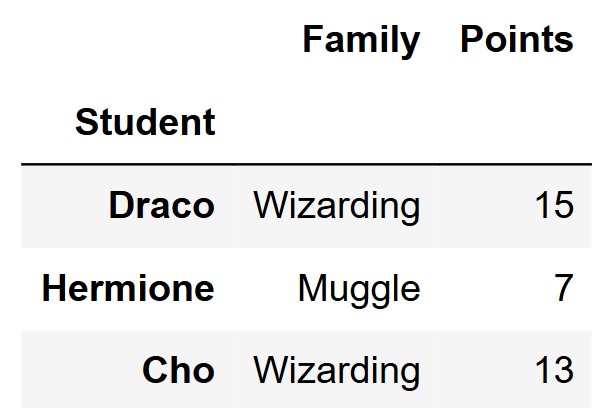
The DataFrame snape is indexed by "Student"
and contains information on each student’s family background
("Family") and the number of house points awarded by Snape
("Points"). The first few rows of snape are
shown below.
Which of the following is the most appropriate test statistic for our permutation test?
The total number of house points awarded to students from wizarding families minus the total number of house points awarded to students from muggle families.
The mean number of house points awarded to students from wizarding families minus the mean number of house points awarded to students from muggle families.
The number of students from wizarding families minus the number of students from muggle families.
The absolute difference between the mean number of house points awarded to students from wizarding families and the mean number of house points awarded to students from muggle families.
Answer: The mean number of house points awarded to students from wizarding families minus the mean number of house points awarded to students from muggle families.
Let’s look at each of the options:
The average score on this problem was 83%.
Fill in the blanks in the function one_stat, which
calculates one value of the test statistic you chose in part (a), based
on the data in df, which will have columns called
"Family" and "Points".
    def one_stat(df):
        grouped = df.groupby(__(a)__).__(b)__
return __(c)__Answer:
"Family"mean()grouped.get("Points").loc["Wizarding"] - grouped.get("Points").loc["Muggle"]
or
grouped.get("Points").iloc[1] - grouped.get("Points").iloc[0]We first group by the "Family" column, which will create
two groups, one for wizarding families and one for muggle families.
Using mean() as our aggregation function here will give
us the mean of each of our two groups, allowing us to prepare for taking
the difference in group means.
The grouped DataFrame will have two rows with
"Wizarding" and "Muggle" as the index, and
just one column "Points" which contains the mean of each
group. We can either use .loc[] or .iloc[] to
get each group mean, and then take the mean number of house points for
wizarding families minus the mean number of house points for muggle
families. Note that we cannot do this the other way around since our
test statistic we chose in part (a) specifically mentions that
order.
The average score on this problem was 81%.
Fill in the blanks in the function calculate_stats,
which calculates 1000 simulated values of the test statistic you chose
in part (a), under the assumptions of the null hypothesis. As before,
df will have columns called "Family" and
"Points".
    def calculate_stats(df)
        statistics = np.array([])

        for i in np.arange(1000):
            shuffled = df.assign(Points = __(d)__)
            stat = one_stat(__(e)__)
            statistics = __(f)__

return statisticsAnswer:
np.random.permutation(df.get("Points"))shufflednp.append(statistics, stat)Since we performing a permutation test, we need to shuffle the
"Points" column to simulate the null hypothesis, that Snape
awards points independently of family background. Note that shuffling
either "Family" or "Points" would work, but in
this case the code specifies that we are naming this shuffled column
Points.
Next, we pass shuffled into our one_stat
function from part (b) to calculate the test statistic for
shuffled.
We then store our test statistic in the statistics
array, which will have 1000 simulated test statistics under the null
hypothesis once the for loop finishes running.
The average score on this problem was 85%.
Fill in the blanks to calculate the p-value of the permutation test,
based on the data in snape.
    observed = __(g)__
    simulated = __(h)__
p_value = (simulated __(i)__ observed).mean()Answer:
one_stat(snape) or
snape.groupby("Family").mean().get("Points").loc["Wizarding"] - snape.groupby("Family").mean().get("Points").loc["Muggle"]
or
snape.groupby("Family").mean().get("Points").iloc[1] - snape.groupby("Family").mean().get("Points").iloc[0]calculate_stats(snape)>=Our observed is going to be the test statistic we obtain from the
initial observed data. We already created a function to calculate the
test statistic — one_stat—, so we just need to apply it to
our observed data —snape—, giving
one_state(snape) in blank g. You can also manually
calculate the observed test statistic by applying the logic in the
formula giving either:
snape.groupby("Family").mean().get("Points").loc["Wizarding"] - snape.groupby("Family").mean().get("Points").loc["Muggle"]
or
snape.groupby("Family").mean().get("Points").iloc[1] - snape.groupby("Family").mean().get("Points").iloc[0].
The simulated variable is simply the array of simulated test
statistics. We already created a function to run the simulation called
calculate_stats, so we just need to call it with our data
giving calculate_stats(snape) in blank h.
Finally, the p-value is the probability of observing a result as
extreme or even more extreme than our observed. The alternative
hypothesis states that Snape awards more points to students from
wizarding families, and the test statistic is the mean points of
wizarding families minus the mean points from muggle families. Thus, in
this case, a more extreme result, would be the simulated statistics
being larger than the observed value. Thus, we use the
>= operator in blank i to calculate the the number of
simulated statistics that are equal to or greater than the observed
value. Calculating the mean of this boolean series will output this
proportion of seeing a result as extreme or even more extreme than the
observed.
The average score on this problem was 80%.
The average score on this problem was 80%.
The average score on this problem was 81%.
Define mini_snape = snape.take(np.arange(3)) as shown
below.

Determine the value of the following expression.
len(calculate_stats(mini_snape))Answer: 1000
This problem is trying to find the length of the
calculate_stats(snape) array. Looking at
calculate_stats, we know that it calculates a simulated
test statistic and appends it to the output array 1000 times as
indicated in the for loop. Thus, the output of the function is an array
of size 1000.
The average score on this problem was 78%.
With mini_snape defined as above, there will be at most
three unique values in calculate_stats(mini_snape). What
are those three values? Put the smallest value on the left and
the largest on the right.
Answer: -5, -2, and 7
We are trying to find the three unique values outputted by
calculate_stats(mini_snape). The function shuffles the
'Points' column, thus assigning new points to either the
‘Wizarding’ or ‘Muggle’ label. We know that there is one ‘Muggle’ label
and two ‘Wizarding’ labels, so with each iteration, the ‘Wizarding’
label will have two items and the ‘Muggle’ label will only have one
item. There are only three unique values that can be calculated from
this because there are only three unique groups of two and one that can
be made using the data. For example, if the data was A,B,C, then the
only three unique groups of two and one we can create are AC and B, AB
and C, and BC and A. Thus, we can now just run through all the
combinations of groups to find our three unique values. We can do this
by forming each scenario of groupings and calculating the test statistic
by finding the mean number of points for ‘Wizarding’ and then
subtracting by the value of ‘Muggle’ as dictated by the test statistic
(Note: we do not need to take a mean for ‘Muggle’ since there is only
one value assigned here):
Scenario 1:
\begin{align*} \frac{15+7}{2} &= 11 \\ 11 - 13 &= -2 \end{align*}
Scenario 2:
Scenario 3:
\begin{align*} \frac{13+15}{2} &= 14 \\ 14 - 7 &= 7 \end{align*}
Thus, our answer from least to greatest is -5, -2, and 7.
The average score on this problem was 66%.
Professor Minerva McGonagall, head of Gryffindor, may also be awarding house points unfairly. For this question, we’ll assume that all four of the houses contain the same number of students, and we’ll investigate whether McGonagall awards points equally to all four houses.
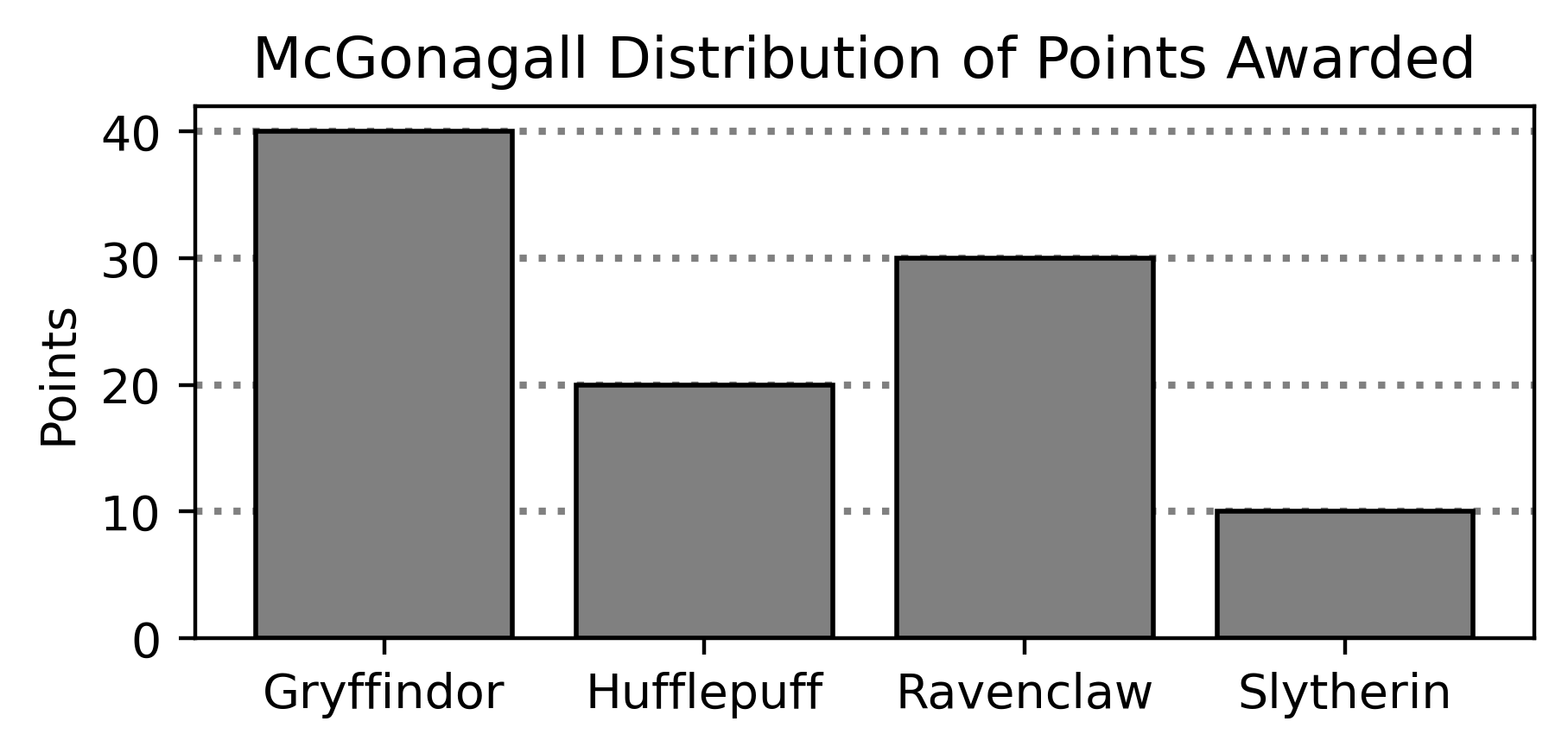
Below is the distribution of points that Professor McGonagall awarded during the last academic year.
You want to test the following hypotheses:
Null Hypothesis: The distribution of points awarded by Professor McGonagall is uniform across all of the houses.
Alternative Hypothesis: The distribution of points awarded by Professor McGonagall is not uniform across all of the houses.
Which of the following test statistics is appropriate for this hypothesis test? Select all that apply.
The absolute difference between the number of points awarded to Gryffindor and the proposed proportion of points awarded to Gryffindor.
The difference between the number of points awarded to the house with the most points and the house with the least points.
The sum of the squared differences in proportions between
McGonagall’s distribution and [0.5, 0.5, 0.5, 0.5].
The sum of the differences in proportions between McGonagall’s
distribution and [0.25, 0.25, 0.25, 0.25].
The sum of the squared differences in proportions between
McGonagall’s distribution and [0.25, 0.25, 0.25, 0.25].
None of the above.
Answer: Option 2 and 5.
This problem is trying to find test statistics that can be used to distinguish when the data is better supported by the alternative. Since the alternative hypothesis simply states “is not uniform across all of the houses”, it is not crucial to look for individual differences between houses but rather the general relationship of points awarded to all houses.
Option 1: This option only tells us information about Gryffindor but doesn’t tell us anything about inequalities between other houses. For example,e if Gryffindor received 25% of the points and Slytherin received the other 75% of the points we would not be able to tell this apart from the case when all houses received 25% of the points.
Option 2: When the points are distributed normally we would expect that all the houses receive about the same amount and therefore the difference of points would be near 0. However, if one house is gaining more points than the rest of the houses then the number of points between the top and lowest house we be greater than 0. Therefore we are “measuring” the alternative.
Option 3: This test statistic measures the sum of
the squared differences in proportions between McGonagall’s distribution
and [0.5, 0.5, 0.5, 0.5]. However,
[0.5, 0.5, 0.5, 0.5] does not represent a valid probability
distribution because the total sum exceeds 1. As a result, this test
statistic is not meaningful in assessing whether the point distribution
is uniform across houses.
Option 4: When we measure the sum of the
differences, the information on “how close” the data is to the
alternative can be unseen. For example, a distribution of
[0.25, 0.25, 0.25, 0.25] is what we’d expect under the null
and a distribution of [0.0, 0.5, 0.0, 0.5] would support
the alternative. However, using this test statistic we would see a
result of 0 therefore not differentiating them.
Option 5: Under the null hypothesis
[0.25, 0.25, 0.25, 0.25] is the “expected” distribution.
Additionally, since the alternative hypothesis states that McGongall’s
assignments are not uniform (aka is the distribution of points
non-uniform), a house supports the alternative if its points are
significantly less than or greater than 0.25.
Squaring the differences allows the test statistic to be greater in
either case and therefore would be a valid statistic.
The average score on this problem was 78%.

For the rest of this problem, we will use the following test statistic:
The sum of the absolute differences in proportions between
McGonagall’s distribution and
[0.25, 0.25, 0.25, 0.25].
Choose the correct way to implement the function
calculate_test_stat, which takes in two distributions as
arrays and returns the value of this test statistic.
    def calculate_test_stat(dist_1, dist_2):
        return _____
np.abs(sum(dist_1 - dist_2)).
abs(sum(dist_1 - dist_2)).
sum(np.abs(dist_1 - dist_2)).
sum(abs(dist_1 - dist_2)).
Answer:
sum(np.abs(dist_1 - dist_2))
A valid test statistic in this problem would find how far
dist_1 differs from dist_2. Since we’re
looking at “how
different” the distributions are, we need to take the absolute value
(aka a measure of distance/difference) and then add them up.
np.abs() needs to be used over abs() because
dist_1 and dist_2 are arrays
and the built-in function abs only works for individual
numbers.
The average score on this problem was 84%.
(10 pts) Fill in the blanks in the code below so that
simulated_ts is an array containing 10,000 simulated values
of the test statistic under the null. Note that your answer to blank
(c) is used in more than one place in the
code.
    mc_gon = np.arange(__(a)__) # Careful: np.arange, not np.array!
    null = np.array([0.25, 0.25, 0.25, 0.25])
    observed_ts = calculate_test_stat(__(b)__)

    simulated_ts = np.array([])

    for i in np.arange(10000):
        sim = np.random.multinomial(__(c)__, __(d)__) / __(c)__
        one_simulated_ts = calculate_test_stat(__(e)__)
        simulated_ts = np.append(simulated_ts, one_simulated_ts)
What goes in blank (a)?
Answer: 0.1, 0.5, 0.1 (or equivalent)
Based on the distribution shown in the bar chart above, we want our
resulting array to contain the proportions
[0.4, 0.2, 0.3, 0.1] (40/100 for Gryffindor, 20/100 for
Hufflepuff, 30/100 for Ravenclaw, and 10/100 for Slytherin). Note that
the order of these proportions does not matter because: 1) we are
calculating the absolute difference between each value and the null
proportion (0.25), and 2) we will sum all the differences together.
Since these proportions are incrementally increasing, we can use
np.arange() to construct mc_gon. There are
multiple correct approaches to this problem, as long as the resulting
array contains all four proportions. Some alternative correct approaches
include: - np.arange(0.4, 0.0, -0.1) -
np.arange(0.1, 0.41, 0.1) (The middle argument can be any
value greater than 0.4 and less than or equal to 0.5)
The average score on this problem was 57%.
What goes in blank (b)?
Answer: null, mc_gon
Note that the order of mc_gon and null does
not matter, as calculate_test_stat calculates the absolute
difference between the two.
The average score on this problem was 78%.
What goes in blank (c)?
Answer: 100
Blank (c) represents the total number of trials in each simulated sample. Using 100 ensures that each sample is large enough to approximate the expected proportions while maintaining computational efficiency. Additionally, (c) is used to divide all values, converting counts into proportions.
The average score on this problem was 48%.
What goes in blank (d)?
Answer: null
Blank (d) is null because each simulated sample is generated under
the null hypothesis. This means the probabilities used in
np.random.multinomial should match the expected proportions
from the null distribution.
The average score on this problem was 77%.
What goes in blank (e)?
Answer: sim, null
Note that the order of null and sim does
not matter, as calculate_test_stat calculates the absolute
difference between the two.
The average score on this problem was 67%.
Fill in the blank so that reject_null evaluates to
True if we reject the null hypothesis at the 0.05 significance level, and
False otherwise.
reject_null = __(f)__Answer:
(simulated_ts >= observed_ts).mean() <= 0.05
reject_null should evaluate to a boolean statement
therefore we must test whether our p-value
is less than or equal to 0.05. Taking the mean of
(simulated_ts >= observed_ts) tells us the proportion of
simulated test statistics that are equal to the value that was observed
in the data or is even further in the direction of the alternative.
The average score on this problem was 64%.
Your friend performs the same hypothesis test as you, but uses the total variation distance (TVD) as their test statistic instead of the one described in the problem. Which of the following statements is true?
Your friend’s simulated statistics will be larger than yours, because TVD accounts for the magnitude and direction of the differences in proportions.
Your friend’s simulated statistics will be larger than yours, but not because it accounts for the magnitude and direction of the differences in proportions.
Your friend’s simulated statistics will be smaller than yours, because TVD accounts for the magnitude and direction of the differences in proportions.
Your friend’s simulated statistics will be smaller than yours, but not because it accounts for the magnitude and direction of the differences in proportions.
There is no relationship between the statistic you used and the statistic your friend used (TVD).
Answer: Option 4.
TVD is calculated by taking the sum of the absolute differences of two proportions, all divided by 2. Therefore the only difference between TVD and our test statistic is the fact that TVD is divided by 2 (which would make it smaller). Meaning that the reason it is smaller is not related to magnitude or direction.
The average score on this problem was 63%.
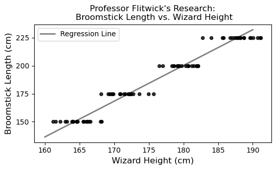
Professor Filius Flitwick is conducting a study whose results will be used to help new Hogwarts students select appropriately sized broomsticks for their flying lessons. Professor Flitwick measures several wizards’ heights and broomstick lengths, both in centimeters. Since broomsticks can only be purchases in specific lengths, the scatterplot of broomstick length vs. height has a pattern of horizontal stripes:
If we group the wizards in Professor Flitwick’s research study by their broomstick length, and average the heights of the wizards in each group, we get the following results.
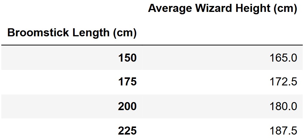
It turns out that the regression line that predicts broomstick length (y) based on wizard height (x) passes through the four points representing the means of each group. For example, the first row of the DataFrame above means that (165, 150) is a point on the regression line, as you can see in the scatterplot.
Based only on the fact that the regression line goes through these points, which of the following could represent the relationship between the standard deviation of broomstick length (y) and wizard height (x)? Select all that apply.
SD(y) = SD(x)
SD(y) = 2\cdot SD(x)
SD(y) = 3\cdot SD(x)
SD(y) = 4\cdot SD(x)
SD(y) = 5\cdot SD(x)
Answer: Options 4 and 5.
To solve this problem, we use the relationship between the slope of the regression line, the correlation coefficient r, and the standard deviations:
\text{slope} = r \cdot \frac{\text{SD}(y)}{\text{SD}(x)}
From the mean points given, we can calculate the slope:
\frac{225 - 150}{187.5 - 165.0} = \frac{75}{22.5} = \frac{10}{3}
We set up the equation:
r \cdot \frac{\text{SD}(y)}{\text{SD}(x)} = \frac{10}{3}
Now consider each option:
If \text{SD}(y) = \text{SD}(x): r = \frac{10}{3} \text{(not valid, since } r > 1\text{)}
If \text{SD}(y) = 2 \cdot \text{SD}(x): r \cdot 2 = \frac{10}{3} \Rightarrow r = \frac{5}{3} \approx 1.67 \quad \text{(not valid, since } r > 1\text{)}
If \text{SD}(y) = 3 \cdot \text{SD}(x): r \cdot 3 = \frac{10}{3} \Rightarrow r = \frac{10}{9} \approx 1.11 \quad \text{(not valid, since } r > 1\text{)}
If \text{SD}(y) = 4 \cdot \text{SD}(x): r \cdot 4 = \frac{10}{3} \Rightarrow r = \frac{10}{12} = \frac{5}{6} \approx 0.833 \quad \text{(valid)}
If \text{SD}(y) = 5 \cdot \text{SD}(x): r \cdot 5 = \frac{10}{3} \Rightarrow r = \frac{10}{15} = \frac{2}{3} \approx 0.667 \quad \text{(valid)}
Therefore, \text{SD}(y) = 4 \cdot \text{SD}(x) and \text{SD}(y) = 5 \cdot \text{SD}(x) are the only valid options.
The average score on this problem was 64%.
Now suppose you know that SD(y) = 3.5 \cdot SD(x). What is the correlation coefficient, r, between these variables? Give your answer as a simplified fraction.
Answer: \frac{20}{21}
We use the formula for slope:
\text{slope} = r \cdot \frac{\text{SD}(y)}{\text{SD}(x)}
From the mean points given, we can calculate the slope:
\frac{225 - 150}{187.5 - 165.0} = \frac{75}{22.5} = \frac{10}{3}
Since \text{SD}(y) = 3.5 \cdot \text{SD}(x), we plug this into the slope formula:
r \cdot 3.5 = \frac{10}{3}
Solving for r:
\begin{align*} r &= \frac{10}{3} \cdot \frac{1}{3.5} \\ &= \frac{10}{3} \cdot \frac{2}{7} \\ &= \frac{20}{21} \end{align*}
The average score on this problem was 56%.
Suppose we convert all wizard heights from centimeters to inches (1 inch = 2.54 cm). Which of the following will change? Select all that apply.
The standard deviation of wizard heights.
The proportion of wizard heights within three standard deviations of the mean.
The correlation between wizard height and broom length.
The slope of the regression line predicting broom length from wizard height.
The slope of the regression line predicting wizard height from broom length.
None of the above.
Answer: Options 1, 4. and 5.
The average score on this problem was 80%.
Suppose we convert all wizard heights and all broomstick lengths from centimeters to inches (1 inch = 2.54 cm). Which of the following will change, as compared to the original data when both variables were measured in centimeters? Select all that apply.
The correlation between wizard height and broom length.
The slope of the regression line predicting broom length from wizard height.
The slope of the regression line predicting wizard height from broom length.
None of the above.
Answer: None of the above
The average score on this problem was 95%.
Professor Flitwick calculates the root mean square error (RMSE) for his regression line to be 36 cm. What does this RMSE value suggest about the accuracy of the regression line’s broomstick length predictions?
The predictions are, on average, 6 cm off from the actual broomstick lengths.
The predictions are, on average, 36 cm off from the actual broomstick lengths.
The predictions are, on average, (36)^2 cm off from the actual broomstick lengths.
Every wizard’s broomstick length differs from the predicted length by 36 cm.
The predictions are more accurate for shorter wizards than taller wizards.
The RMSE does not tell us anything about prediction accuracy.
None of the above.
Answer: None of the above
RMSE is the square root of the average squared differences between predicted and actual values. None of the options accurately describes what RMSE represents because:
RMSE gives us the typical size of the error in the same units as the response variable. It tells us that the typical prediction error is around 36 cm, but this is not the same as any of the given options.
The average score on this problem was 7%.
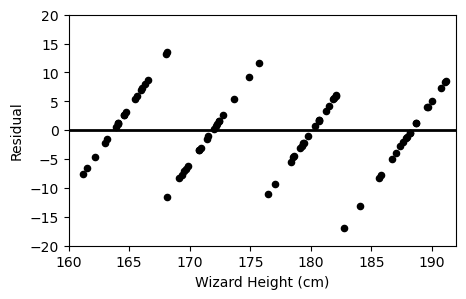
Which of the following plots is the residual plot for Professor Flitwick’s data?
Option A:
Option B:
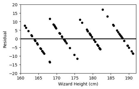
Option C:
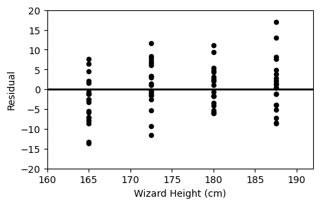
Answer: Option B
A residual plot shows the difference between actual and predicted values plotted against the predictor variable (x).
Since broomsticks come in specific sizes (150, 175, 200, 225 cm), the residuals will form slanted lines across the x axis.
We can immediately rule out Option C, as all the points lie on 4 specific wizard heights, which is totally different from the original plot.
Now, if we were to pick a point:
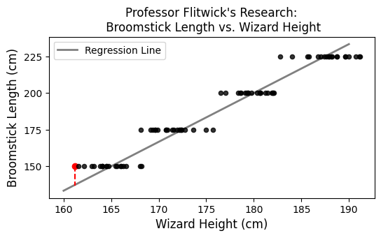 ,
,
We see that this point is above the line, meaning the difference between actual and predicted is positive (actual - predicted > 0)
Thus, if we were to check the point on option A or B, we see that option B’s graph corresponds with the original.
Option A

Option B
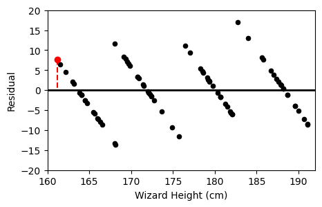 ,
,
The average score on this problem was 59%.
The Triwizard Tournament is an international competition between three wizarding academies: Hogwarts, Durmstrang, and Beauxbatons.
In a Triwizard Tournament, wizards from each school compete in three dangerous magical challenges. If one school wins two or more challenges, that school is the tournament champion. Otherwise, there is no champion, since each school won a single challenge.
The DataFrame triwiz has a row for each challenge from
the first 20 Triwizard Tournaments. With 20 tournaments each having 3
challenges, triwiz has exactly 60 rows.
The first six rows are shown below.
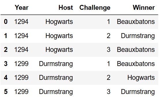
The columns are:
"Year" (int): Triwizard Tournaments are held only
once every five years.
"Host" (str): Triwizard Tournaments are held at one
of the three participating schools on a rotating basis: Hogwarts,
Durmstrang, Beauxbatons, back to Hogwarts again, etc.
"Challenge" (int): Either 1,
2, or 3.
"Winner" (str): The school that won the
challenge.
(10 pts) Fill in the blanks below to create the DataFrame
champions, which is indexed by "Winner" and
has just one column, "Year", containing the number
of years in which each school was the tournament champion.
champions is shown in full below.
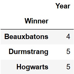
Note that the values in the "Year" column add up to 14,
not 20. That means there were 6 years in which there was a tie (for
example, 1299 was one such year).
    grouped = triwiz.groupby(__(a)__).__(b)__.__(c)__
    filtered = grouped[__(d)__]
    champions = filtered.groupby(__(e)__).__(f)__.__(g)__
What goes in blank (a)?
Answer: ["Year", "Winner"] or
["Winner", "Year"]
Grouping by both the "Year" and "Winner"
columns ensures that each school’s win in a given year is represented as
a single row.
The average score on this problem was 89%.
What goes in blank (b)?
Answer: count()
Since each winner in a given year appears as a single row, we use
count() to determine how many times each school won that
year.
The average score on this problem was 90%.
What goes in blank (c)?
Answer: reset_index()
Grouping by multiple columns creates a multi-index.
reset_index() flattens the DataFrame back to normal, where
each row represents a given year for each winning school.
The average score on this problem was 80%.
What goes in blank (d)?
Answer: grouped.get("Host") != 1 or
grouped.get("Host") > 1 or
grouped.get("Host") >= 2
The Triwizard Tournament winner is defined as a school that wins two
or more challenges in a given year. After grouping with
.count(), all other columns contain the same value, which
is the number of challenges each winning school won
that year. A school will not appear in this DataFrame if they did not
win any challenges that year, so we only need to check if the value in
the other columns is not 1.
.get("Challenge") is also valid because all other columns
contain the same value.
The average score on this problem was 71%.
What goes in blank (e)?
Answer: "Winner"
The resulting DataFrame should be indexed by "Winner",
therefore the DataFrame is grouped by the "Winner"
column.
The average score on this problem was 90%.
What goes in blank (f)?
Answer: count()
Grouping with .count() again ensures that the resulting
columns represent the number of times each "Winner"
(school) in the index won across all years.
The average score on this problem was 84%.
What goes in blank (g)?
Answer: get(["Year"])
The question asks for a DataFrame with "Year" as the
only column, so brackets are used around "Year" to ensure
the output is a DataFrame rather than a Series.
The average score on this problem was 69%.
How many rows are in the DataFrame that results from merging
triwiz with itself on "Year"? Give your answer
as an integer.
Answer: 180
The most important part of this question is understanding how
merge works in babypandas. Start by
reviewing this diagram
from lecture.
When we merge two DataFrames together by "Year", we are
matching every row in triwiz with every other row that has
the same value in the "Year" column. This means that for
each year, we’ll match all the rows from that year with each other.
Since there are three challenges per year, that means that each year
appears 3 times in the DataFrame. Since we are matching all rows from
each year with each other, this means we will end up with 3 * 3 or 9 rows per year. Since there are 20
years in the DataFrame, we can multiply these together to get 180 total
rows in the merged DataFrame.
The average score on this problem was 69%.
How many rows are in the DataFrame that results from merging
triwiz with itself on "Challenge"? Give your
answer as an integer.
Answer: 1200
Similar to the previous part, we are now matching all rows from a
given challenge to each other. There are 3 challenges per tournament, so
the values in the "Challenge" column are 1,
2, and 3. Each such values appears 20 times,
once for each year. As a result, for each of the 3 challenges there are
20 * 20 or 400 rows. Therefore, we have
400 * 3 = 1200 rows total.
The average score on this problem was 59%.
How many rows are in the DataFrame that results from merging
triwiz with itself on "Host"? Select the
expression that evaluates to this number.
2\cdot 6^2 + 7^2
2\cdot 7^2 + 6^2
2\cdot 18^2 + 21^2
2\cdot 21^2 + 18^2
Answer: 2 * 21^2 + 18^2
The key to understanding how this problem works is by understanding how many times each school ends up hosting the tournament within this dataset. It is stated that the host is determined on a rotating basis. Based on the DataFrame description, we know the order is Hogwarts, Durmstrang, and then Beauxbatons. Since there are only 20 years in this dataset, the last school in the rotation will have one less host than the other two schools. Thus, we have determined that Hogwarts hosts 7 times, Durmstrang hosts 7 times, and Beauxbatons hosts 6 times. Since for each year a school hosts, they appear three times in the DataFrame, each school appears 21 times, 21 times, and 18 times respectively. As stated in the above questions when merging we are matching all rows from a given host to each other. Therefore, the total rows can be expressed as 21^2 + 21^2 + 18^2. This matches the last answer choice.
The average score on this problem was 43%.
Bertie Bott’s Every Flavor Beans are a popular treat in the wizarding world. They are jellybean candies sold in boxes of 100 beans, containing a variety of flavors including chocolate, peppermint, spinach, liver, grass, earwax, and paper. Luna’s favorite flavor is bacon.
Luna wants to estimate the proportion of bacon-flavored beans produced at the Bertie Bott’s bean factory. She buys a box of Bertie Bott’s Every Flavor Beans and finds that 4 of the 100 beans inside are bacon-flavored. Using this sample, she decides to construct an 86\% CLT-based confidence interval for the proportion of bacon-flavored beans produced at the factory.
Let’s begin by solving a related problem that will help us in the later parts of this question. Consider the following fact:
For a sample of size 100 consisting of 0’s and 1’s, the maximum possible width of an 86\% CLT-based confidence interval is approximately 0.15.
Use this fact to find the value of z such that
scipy.stats.norm.cdf(z) evaluates to 0.07.
Give your answer as a number to one decimal place.
Answer: -1.5
The 86% confidence interval for the population mean is given by:
\left[ \text{sample mean} - |z| \cdot \frac{\text{sample SD}}{\sqrt{\text{sample size}}}, \ \text{sample mean} + |z| \cdot \frac{\text{sample SD}}{\sqrt{\text{sample size}}} \right]
Since the width is equal to the difference between the right and left endpoints,
\text{width} = 2 \cdot |z| \cdot \frac{\text{sample SD}}{\sqrt{\text{sample size}}}
We solve for |z|. The maximum width of our CI is given to be 0.15, so we must also use the maximum possible standard deviation, 0.5. we substitute the known values to obtain:
0.15 = 2 \cdot |z| \cdot \frac{0.5}{\sqrt{100}}
which leaves |z| = 1.5 after
computation. To find the z such that
scipy.stats.norm.cdf(z) evaluates to 0.07, we
realize that z is the point under the
normal curve, in standard units, left of which represents 7\% of the area under the entire curve. Note
that scipy.stats.norm.cdf(0) evaluates to 0.5
(Recall: half of the area is left of the mean, which is zero in standard
units). We must therefore take a negative value for z. Thus z =
-1.5.
The average score on this problem was 55%.
Suppose that Luna’s sample has a standard deviation of 0.2. What are the endpoints of her 86\% confidence interval? Give each endpoint as a number to two decimal places.
Answer: [0.01, \ 0.07]
Recall the formula for the width of an 86\% confidence interval:
\text{width} = 2 \cdot |z| \cdot \frac{\text{sample SD}}{\sqrt{\text{sample size}}}
where we found |z| = 1.5 in part (a). Instead of using the maximum sample SD, we will now use 0.2 and compute the new width of the confidence interval. This results in
\text{width} = 2 \cdot 1.5 \cdot \frac{0.2}{\sqrt{10}} = 0.06
Since this is a CLT-based confidence interval for the population mean, the interval must be centered at the mean. We compute the interval using the structure from part (a), which leaves
\left[ 0.04 - \frac{1}{2} \cdot 0.06, \ 0.04 + \frac{1}{2} \cdot 0.06 \right] = [0.01, \ 0.07]
The average score on this problem was 37%.
Hermione thinks she can do a better job of estimating the proportion of bacon-flavored beans, though she’ll need a bigger sample to do so. Hermione will collect a new sample and use it to construct another 86\% confidence interval for the same parameter.
Under the assumption that Hermione’s sample will have the same standard deviation as Luna’s sample, which was 0.2, how many boxes of Bertie Bott’s Every Flavor Beans must Hermione buy to guarantee that the width of her 86\% confidence interval is at most 0.012? Give your answer as an integer.
Remember: There are 100 beans in each box.
Answer: 25 boxes
Recall the formula for the width of an 86\% confidence interval:
\text{width} = 2 \cdot |z| \cdot \frac{\text{sample SD}}{\sqrt{\text{sample size}}}
where we must again use the fact that |z| = 1.5 from part (a). Here, we want a width that is no larger than 0.012, given that our sample SD remains 0.2. Plugging everything in:
0.012 \geq 2 \cdot 1.5 \cdot \frac{0.2}{\sqrt{n}}
Rearranging the expression to solve for n, we get
\begin{align*} n &\geq \left( \frac{3 \cdot 0.2}{0.012} \right)^2 \\ n &\geq \left( \frac{600}{12} \right)^2 \\ n &\geq (50)^2 \\ n &\geq 2500 \end{align*}
However, 2500 isn’t our final answer. The question asks for the number of boxes Hermione must buy, given that each box contains 100 beans. The bound we computed above for n corresponds to the minimum number of beans Hermione must observe. To get the minimum number of boxes, we simply divide the bound by 100. The final answer is 25 boxes.
The average score on this problem was 37%.