← return to practice.dsc10.com
Instructor(s): Janine Tiefenbruck
This exam was administered in-person. Students were allowed one page of double-sided handwritten notes. No calculators were allowed. Students had 50 minutes to take this exam.
⚠️ PDF version available here .
Note (groupby / pandas 2.0): Pandas 2.0+ no longer
silently drops columns that can’t be aggregated after a
groupby, so code written for older pandas may behave
differently or raise errors. In these practice materials we use
.get() to select the column(s) we want after
.groupby(...).mean() (or other aggregations) so that our
solutions run on current pandas. On real exams you will not be penalized
for omitting .get() when the old behavior would have
produced the same answer.
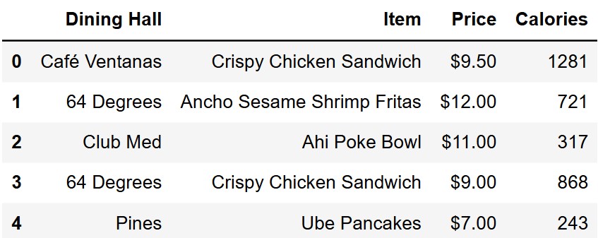
In this exam, you’ll work with a data set showcasing the different
dining halls at UCSD and the foods served there. Each row represents a
single menu item available at one of the UCSD dining halls. The columns
of dining are as follows:
• "Dining Hall" (str): The name of the
dining hall.
• "Item" (str): The name of the menu
item.
• "Price" (str): The cost of the menu
item.
• "Calories" (int): The number of calories
in the menu item.
The rows of dining are in no particular order. The first
few rows are shown below, though dining has many more rows
than pictured.
Which of the following columns would be an appropriate index for the
dining DataFrame?
"Dining Hall"
"Item"
"Price"
"Calories"
None of these.
Answer: None of these
None of the following columns would be an appropriate index since
they all possibly contain duplicates. We are told that each row
represents a single menu item available at one of the UCSD dining halls.
This means that each row represents a combination of both
"Dining Hall" and "Item" so no one column is
sufficient to uniquely identify a row. We can see this in the preview of
the first few rows of the DataFrame. There are multiple rows with the
same value in the "Dining Hall" column, and also multiple
rows with the same value in the "Item" column.
While "Price" and "Calories" could
be unique, it doesn’t make sense to refer to a row by its price or
number of calories. Further, we have no information that guarantees the
values in these columns are unique (they’re probably not).
The average score on this problem was 76%.
As a broke college student, you are on a mission to find the dining hall with the greatest number of affordable menu items.
To begin, you want a DataFrame with the same columns as
dining, but with an additional column
"Affordability" which classifies each menu item as
follows:
"Cheap", for items that cost $6 or less.
"Moderate", for items that cost more than $6 and at
most $14.
"Expensive", for items that cost more than
$14.
Fill in the blanks below to assign this new DataFrame to the variable
with_affordability.
    def categorize(price):
        price_as_float = __(a)__
        if price_as_float __(b)__:
            return __(c)__
        elif price_as_float > 6:
            return "Moderate"
        else:
            return __(d)__
with_affordability = dining.assign(Affordability = __(e)__)Answer (a): float(price.strip("$")) or
float(price.replace("$", "")) or
float(price.split("$")[1])
To solve this problem, we must keep in mind that the prices in the
"Price" column are formatted as strings with dollar signs
in front of them. For example, we might see a value such as
"$9.50". Our function’s goal is to transform any given
value in the "Price" column into a float matching the
corresponding dollar amount.
Therefore, one strategy is to first use the .strip
string method to strip the price of the initial dollar sign. Since we
need our output as a float, we can call the python float
function on this to get the price as a float.
The other strategies are similar. We can replace the dollar sign with
the empty string, effectively removing it, then convert to a float.
Similarly, we can split the price according to the instances of
"$". This will return a list of two elements, the first of
which contains everything before the dollar sign, which is the empty
string, and the second of which contains everything after the dollar
sign, which is the part we want. We extract it with [1] and
then convert the answer to a float.
The average score on this problem was 61%.
Answer (b): > 14
The key to getting this question correct comes from understanding how
the placement of price_as_float > 6 affects how you
order the rest of the conditionals within the function. The method
through which we test if a price is "Moderate" is by
checking if price_as_float > 6. But
"Moderate" is defined as being not only more than 6 dollars
but also less that or equal to 14 dollars. So we must first check to see
if the price is "Expensive" before we check and see if the
price is "Moderate". This way, prices that are in the
"Expensive" range get caught by the first if
statement, and then prices in the "Moderate" range get
caught by the elif.
The average score on this problem was 74%.
Answer (c): "Expensive"
In the previous part of this question we checked to see if the
price_as_float > 14. We did this to see if the given
price falls into the "Expensive" category. Since the
categorize function is meant to take in a price and output
the corresponding category, we just need to output the correct category
for this conditional which is "Expensive".
The average score on this problem was 75%.
Answer (d): "Cheap"
In the previous parts of this question, we have implemented checks to
see if a price is "Expensive" or "Moderate".
This leaves only the "Cheap" price category, meaning that
it can be placed in the else statement. The logic is we check if a price
is "Expensive" or "Moderate" and if its
neither, it has to be "Cheap".
The average score on this problem was 74%.
Answer (e):
dining.get("Price").apply(categorize)
Now that we have implemented the categorize function, we
need to apply it to the "Price" column so that it can be
added as a new column into dining. Keep in mind our
function takes in one price and outputs its price category. Thus, we
need a way to apply this function to every value in the Series that
corresponds to the "Price" column. To do this, we first
need to get the Series from the DataFrame and then use
apply on that Series with our categorize
function as the input.
The average score on this problem was 89%.
Now, you want to determine, for each dining hall, the number of menu
items that fall into each affordability category. Fill in the blanks to
define a DataFrame called counts containing this
information. counts should have exactly three columns,
named "Dining Hall", "Affordability", and
"Count".
    counts = with_affordability.groupby(__(f)__).count().reset_index()
counts = counts.assign(Count=__(g)__).__(h)__Answer (f):
["Dining Hall", "Affordability"] or
["Affordability", "Dining Hall"]
The key to solving this problem comes from understanding exactly what
the question is asking. You are asked to create a DataFrame that
displays, in each dining hall, the number of menu items that fall into
each affordability category. This indicates that you will need to group
by both “Dining Hall” and “Affordability” because when you group by
multiple columns you get a row for every combination of values in those
columns. Remember that to group by multiple columns, you need to input
the columns names in a list as an argument in the
groupby function. The order of the columns does not
matter.
The average score on this problem was 81%.
Answer (g): counts.get("Price") or
counts.get("Calories") or
counts.get("Item")
For this part, you need to create a column called
"Count" with the number of menu items that fall into each
affordability category within each dining hall. The
.count() aggregation method works by counting the number of
values in each column within each group. In the resulting DataFrame, all
the columns have the same values, so we can use the values from any one
of the non-index columns in the grouped DataFrame. In this case, those
columns are "Price", "Calories", and
"Item". Therefore to fill in the blank, you would get any
one of these columns.
The average score on this problem was 62%.
Answer (h):
get(["Dining Hall", "Affordability", "Count"])or
drop(columns=["Item", "Price", "Calories"]) (columns can be
in any order)
Recall the question asked to create a DataFrame with only three
columns. You have just added one of the columns, "Count.
This means you have to drop the remaining columns ("Price",
"Calories", and "Item") or simply get the
desired columns ("Dining Hall",
"Affordability", and "Count").
The average score on this problem was 77%.
Suppose you determine that "The Bistro" is the dining
hall with the most menu items in the "Cheap" category, so
you will drag yourself there for every meal. Which of the following
expressions must evaluate to the number of "Cheap" menu
items available at "The Bistro"? Select all that
apply.
counts.sort_values(by="Count", ascending=False).get("Count").iloc[0]
counts.get("Count").max()
(counts[counts.get("Affordability") == "Cheap"].sort_values(by="Count").get("Count").iloc[-1])
counts[counts.get("Dining Hall") == "The Bistro"].get("Count").max()
counts[(counts.get("Affordability") == "Cheap") & (counts.get("Dining Hall") == "The Bistro")].get("Count").iloc[0]
None of these.
Answer:
(counts[counts.get("Affordability") == "Cheap"].sort_values(by="Count").get("Count").iloc[-1])
and
counts[(counts.get("Affordability") == "Cheap") & (counts.get("Dining Hall") == "The Bistro")].get("Count").iloc[0]
Option 1: This code sorts all rows by
"Count" in descending order (largest to smallest) and
selects the count from the first row. This is incorrect because there
can be another combination of "Dining Hall" and
"Affordability" that has a number of menu items larger than
the number of "Cheap" items at "The Bistro".
For example, maybe there are 100 "Cheap" items at
"The Bistro" but 200 "Moderate" items at
"Pines".
Option 2: This code selects the largest value in
the "Count" column, which may not necessarily be the number
of "Cheap" items at "The Bistro". Taking the
same example as above, maybe there are 100 "Cheap" items at
"The Bistro" but 200 "Moderate" items at
"Pines".
Option 3: This code first filters
counts to only include rows where
"Affordability" is "Cheap". Then, it sorts by
"Count" in ascending order (smallest to largest). Since the
question states that "The Bistro" has the most
"Cheap" menu items, selecting the last row
(iloc[-1]) from the "Count" column correctly
retrieves the number of "Cheap" menu items at
"The Bistro".
Option 4: This code filters counts
to only include rows where "Dining Hall" is
"The Bistro", then returns the maximum value in the
"Count" column. However, "The Bistro" may have
more menu items in the "Moderate" or
"Expensive" categories than it does in the
"Cheap" category. This query does not isolate
"Cheap" items, so it incorrectly returns the highest count
across all affordability levels rather than just
"Cheap".
For example, if "The Bistro" has 100
"Cheap" menu items, 200 "Moderate" menu items,
and 50 "Cheap" menu items, this code would evaluate to 200,
even though that is not the number of "Cheap" items at
"The Bistro". This is possible because we are told that
"The Bistro" is the dining hall with the most menu items in
the "Cheap" category, meaning in this example that every
other dining hall has fewer than 100 "Cheap" items.
However, this tells us nothing about the number of menu items at
"The Bistro" in the other affordability categories, which
can be greater than 100.
"Cheap" affordabaility, and a
"Dining Hall" value of "The Bistro". This is
only one such row! The code then selects the first (and only) value in
the "Count" column, which correctly evaluates to the number
of "Cheap" items at "The Bistro".
The average score on this problem was 84%.
Suppose we have access to another DataFrame called
orders, containing all student dining hall orders from the
past three years. orders includes the following columns,
among others:
"Dining Hall" (str): The dining hall
where the order was placed.
"Start" (str): The time the order was
placed.
"End" (str): The time the order was
completed.
All times are expressed in 24-hour military time format (HH:MM). For
example, "13:15" indicates 1:15 PM. All orders were
completed on the same day as they were placed, and "End" is
always after "Start".
Fill in the blanks in the function to_minutes below. The
function takes in a string representing a time in 24-hour military time
format (HH:MM) and returns an int representing the number of minutes
that have elapsed since midnight. Example behavior is given below.
    >>> to_minutes("02:35")
    155

    >>> to_minutes("13:15")
    795

    def to_minutes(time):
        separate = time.__(a)__
        hour = __(b)__
        minute = __(c)__
return __(d)__Answer (a): split(":")
We first want to separate the time string into hours and minutes, so
we use split(":") to turn a string like
"HH:MM" into a list of the form
["HH", "MM"].
The average score on this problem was 84%.
Answer (b): separate[0] or
int(separate[0])
The hour will be the first element of the split list, so we can
access it using separate[0]. This is a string, which we can
convert to an int now, or later in blank (d).
The average score on this problem was 73%.
Answer (c): separate[1] or
int(separate[1])
The minute will be the second element of the split list, so we can
access it using separate[1] or separate[-1].
Likewise, this is also a string, which we can convert to an
int now, or later in blank (d).
The average score on this problem was 73%.
Answer (d):
int(hour) * 60 + int(minute) or
hour * 60 + minute (depending on the answers to (b) and
(c))
In order to convert hours and minutes into minutes since midnight, we
have to multiply the hours by 60 and add the number of minutes. These
operations must be done with ints, not strings.
The average score on this problem was 73%.
Fill in the blanks below to add a new column called
"Wait" to orders, which contains the number of
minutes elapsed between when an order is placed and when it is
completed. Note that the first two blanks both say (e)
because they should be filled in with the same value.
    start_min = orders.get("Start").__(e)__
    end_min = orders.get("End").__(e)__
orders = orders.assign(Wait = __(f)__)Answer (e): apply(to_minutes)
In order to find the time between when an order is placed and
completed, we first need to convert the "Start" and
"End" times to minutes since midnight, so that we can
subtract them. We apply the function we wrote in Problem 3.1 to get the
values of "Start" and "End" in minutes elapsed
since midnight.
The average score on this problem was 87%.
Answer (f): end_min - start_min
Now that we have the values of "Start" and
"End" columns in minutes, we simply need to subtract them
to find the wait time. Note that we are subtracting two Series here, so
the subtraction happens element-wise by matching up corresponding
elements.
The average score on this problem was 87%.
You were told that "End" is always after
"Start" in orders, but you want to verify if
this is correct. Fill the blank below so that the result is
True if "End" is indeed always after
"Start", and False otherwise.
(orders.get("Wait") > 0).sum() == __(g)__Answer (g): orders.shape[0]
Since "Wait" was already calculated in the previous
question by subtracting "End" minus "Start",
we know that positive values indicate where "End" is after
"Start". When we evaluate
orders.get("Wait") > 0, we get a Boolean Series where
True indicates rows where "End" is after
"Start". Taking the .sum() of this Boolean
Series counts how many rows satisfy this condition, using the fact that
True is 1 and False is
0 in Python. If "End" is always after
"Start", this sum should equal the total number of rows in
the DataFrame, which is orders.shape[0]. Therefore,
comparing the sum to orders.shape[0] will return
True exactly when "End" is after
"Start" for all rows.
The average score on this problem was 36%.
Fill in the blanks below so that ranked evaluates to an
array containing the names of the dining halls in orders,
sorted in descending order by average wait time.
    ranked = np.array(orders.__(h)__
                             .sort_values(by="Wait", ascending=False)
.__(i)__)Answer (h):
groupby('Dining Hall').mean()
Since we want to compare the average wait time for each Dining Hall
we know we need to aggregate each Dining Hall and find the mean of the
"Wait" column. This can be done using
groupby('Dining Hall').mean().
The average score on this problem was 62%.
Answer (i): index or
reset_index().get('Dining Hall')
The desired output is an array with the names of
each dining hall. After grouping and sorting, the dining hall names
become the index of our DataFrame. Since we want an array of these names
in descending order of wait times, we can either use .index
to get them directly, or reset_index().get("Dining Hall")
to convert the index back to a column and select it.
The average score on this problem was 43%.
What would be the most appropriate type of data visualization to compare dining halls by average wait time?
scatter plot
line plot
bar chart
histogram
overlaid plot
Answer: bar chart
"Dining Hall" is a categorical variable and the average
wait time is a numerical variable, so a bar chart should be used. Our
visualization would have a bar for each dining hall, and the length of
that bar would be proportional to the average wait time.
The average score on this problem was 89%.
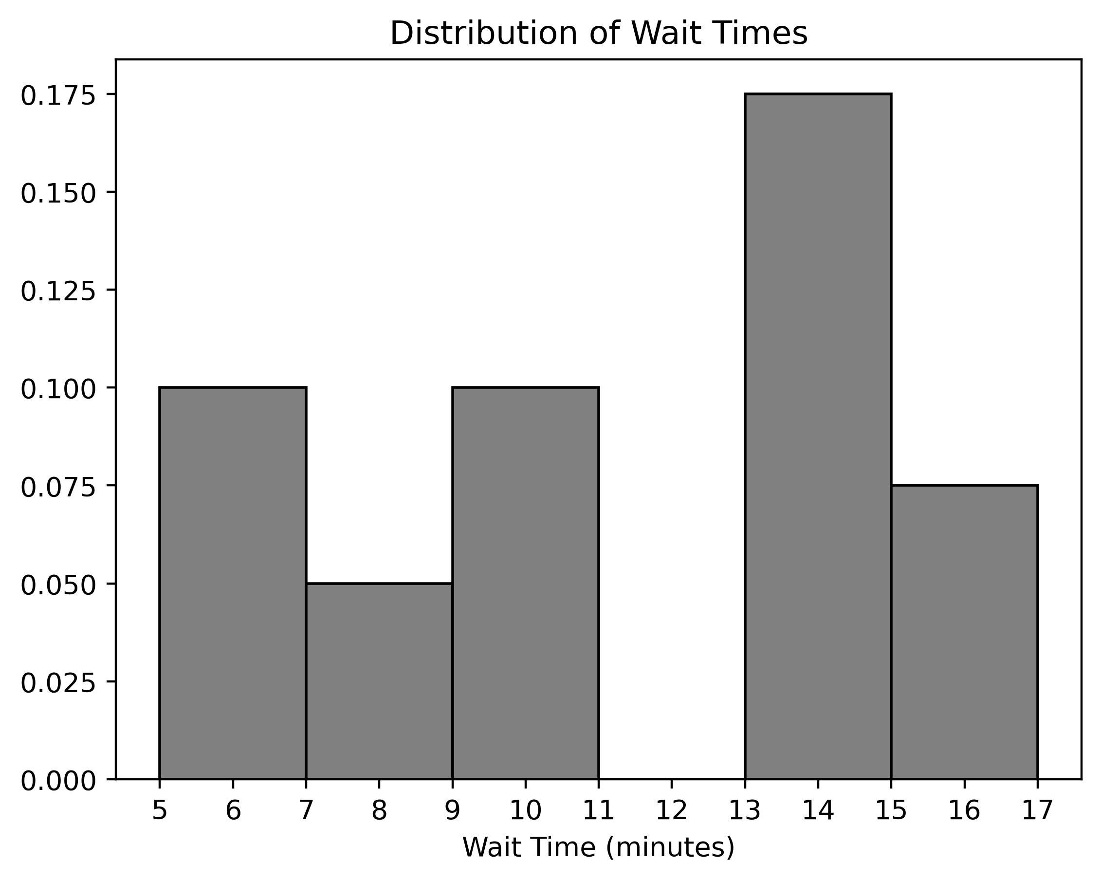
Below is a density histogram displaying the distribution of wait times for orders from UCSD dining halls.
Fill in the blanks to define a variable bins that could
have been used as the bins argument in the call to
.plot that generated the histogram above.
bins = 0.5 * (2 + np.arange(__(a)__, __(b)__, __(c)__))Answer (a): 8
The first piece of information to note is what the bins are in the
original histogram; if we know where we need to arrive at the end of the
problem, it is much easier to piece together the arguments we need to
pass to np.arange in the code provided.
With this in mind, the bins in the original histogram are defined by
the array with values [5, 7, 9, 11, 13, 15, 17]. So, we can
work backwards from here to answer this question.
The final step in the code is multiplying the result of
2 + np.arange(a, b, c) by 0.5. Since we know
this must result in [5, 7, 9, 11, 13, 15, 17], the array
generated by 2 + np.arange(a, b, c) must have the values
[10, 14, 18, 22, 26, 30, 34].
Using similar logic, we know that 2 + np.arange(a, b, c)
must give us the array with values
[10, 14, 18, 22, 26, 30, 34]. By subtracting two, we get
that np.arange(a, b, c) must have values
[8, 12, 16, 20, 24, 28, 32].
There are multiple calls to np.arange() that result in
this sequence. We should start at 8 and step by
4, but where we stop can be any number larger than
32, and at most 36, as this argument is
exclusive and not included in the output array. So, the answers are (a)
= 8, (b) = any number larger than 32 and less
than or equal to 36, and (c) = 4.
The average score on this problem was 68%.
Answer (b): any number in the interval
(32, 36]
Refer to explanation for (a).
The average score on this problem was 56%.
Answer (c): 4
Refer to explanation for (a).
The average score on this problem was 36%.
What proportion of orders took at least 7 minutes but less than 12 minutes to complete?
Answer: 0.3 or 30%
In a density histogram, the proportion of data in a bar or set of bars is equal to the area of those bars. So, to find the proportion of orders that took between 7 and 12 minutes to complete, we must find the area of the bars that encapsulate this range.
The bars associated with the bins [7, 9) and [9, 11) contain all of the orders that took between 7 and 12 minutes. So, summing the areas of these bars tells us the proportion of orders that took between 7 and 12 minutes.
The width of each bar is 2, and the heights of the bars are 0.05 and 0.1, respectively. So, the sum of their areas is 2 \cdot 0.05 + 2 \cdot 0.1 = 0.1 + 0.2 = 0.3. So, 0.30 or 30\% of our orders took between 7 and 12 minutes to complete.
The average score on this problem was 82%.
After some investigation, HDH discovers that every order that took longer than 12 minutes to complete was ordered from The Bistro. As a result, they fire all the employees at The Bistro and permanently close the dining hall. With this update, we generate a new density histogram displaying the distribution of wait times for orders from the other UCSD dining halls.
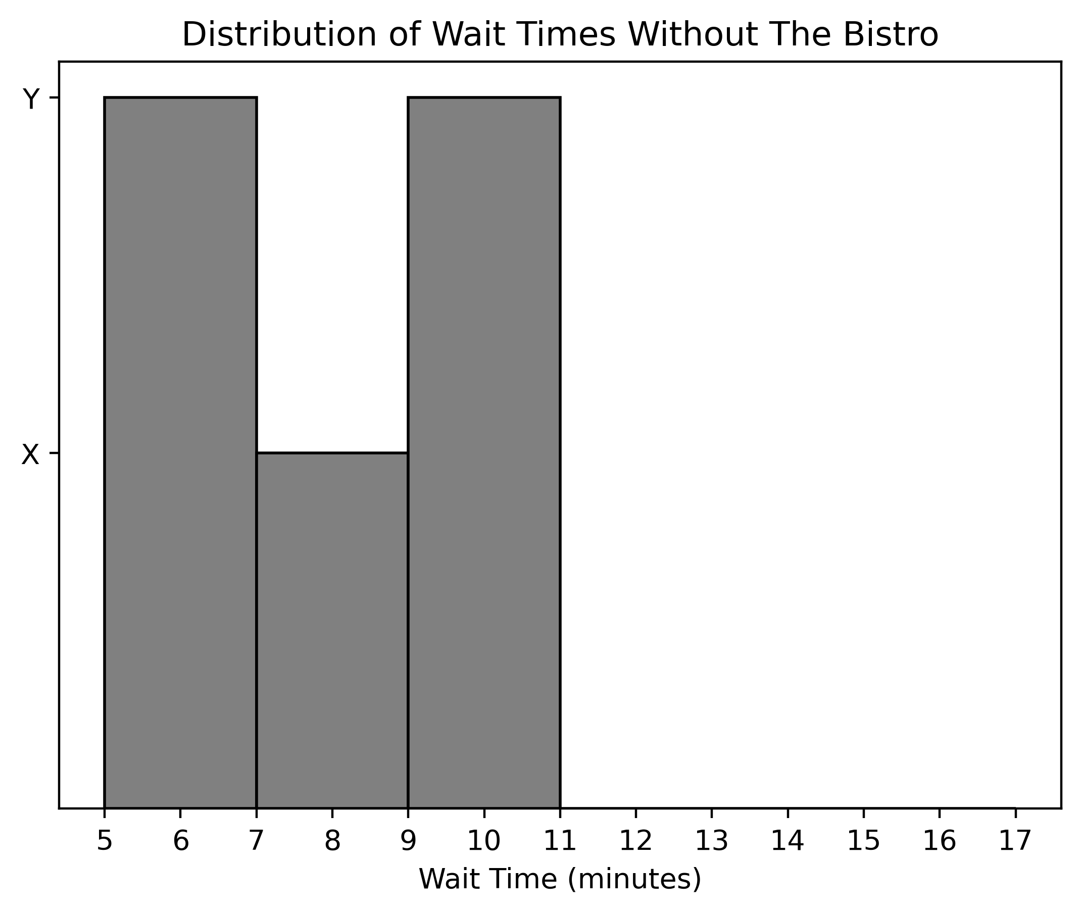
What are the values of X and Y along the y-axis of this histogram?
Answer: X = 0.1, Y = 0.2
The original histogram, including The Bistro’s data, showed a
cumulative density of 0.5 for the first three bars covering
wait times from 5 to 11 minutes. The densities were calculated as:
After we removed The Bistro’s data, these wait time intervals (5 to
11 minutes) now account for the entirety of the dataset. Hence, to
reflect the new total (100% of the data), the original bar heights need
to be doubled, as they previously summed up to 0.5 (or 50%
of the data).
Thus, the new calculation for total density is: 2 \times 0.2 + 2 \times 0.1 + 2 \times 0.2 = 1.0.
The average score on this problem was 53%.
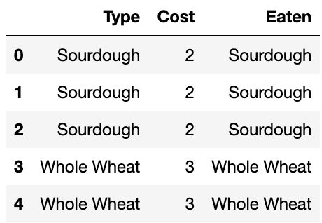
It’s the grand opening of UCSD’s newest dining attraction: The Bread Basket! As a hardcore bread enthusiast, you celebrate by eating as much bread as possible. There are only a few menu items at The Bread Basket, shown with their costs in the table below:
| Bread | Cost |
|---|---|
| Sourdough | 2 |
| Whole Wheat | 3 |
| Multigrain | 4 |
Suppose you are given an array eaten containing the
names of each type of bread you ate.
For example, eaten could be defined as follows:
    eaten = np.array(["Whole Wheat", "Sourdough", "Whole Wheat",
                      "Sourdough", "Sourdough"])
In this example, eaten represents five slices of bread
that you ate, for a total cost of \$12.
Pricey!
In this problem, you’ll calculate the total cost of your bread-eating
extravaganza in various ways. In all cases, your code must calculate the
total cost for an arbitrary eaten array, which might not be
exactly the same as the example shown above.
One way to calculate the total cost of the bread in the
eaten array is outlined below. Fill in the missing
code.
    breads = ["Sourdough", "Whole Wheat", "Multigrain"]
    prices = [2, 3, 4]
    total_cost = 0
    for i in __(a)__:
        total_cost = (total_cost +
np.count_nonzero(eaten == __(b)__) * __(c)__)Answer (a): [0, 1, 2] or
np.arange(len(bread)) or range(3) or
equivalent
Let’s read through the code skeleton and develop the answers from
intuition. First, we notice a for loop, but we don’t yet
know what sequence we’ll be looping through.
Then we notice a variable total_cost that is initalized
to 0. This suggests we’ll use the accumulator pattern to
keep a running total.
Inside the loop, we see that we are indeed adding onto the running
total. The amount by which we increase total_cost is
np.count_nonzero(eaten == __(b)__) * __(c)__. Let’s
remember what this does. It first compares the eaten array
to some value and then counts how many True values are in
resulting Boolean array. In other words, it counts how many times the
entries in the eaten array equal some particular value.
This is a big clue about how to fill in the code. There are only three
possible values in the eaten array, and they are
"Sourdough", "Whole Wheat", and
"Multigrain". For example, if blank (b) were filled with
"Sourdough", we would be counting how many of the slices in
the eaten array were "Sourdough". Since each
such slice costs 2 dollars, we could find the total cost of all
"Sourdough" slices by multiplying this count by 2.
Understanding this helps us understand what the code is doing: it is
separately computing the cost of each type of bread
("Sourdough", "Whole Wheat",
"Multigrain") and adding this onto the running total. Once
we understand what the code is doing, we can figure out how to fill in
the blanks.
We just discussed filling in blank (b) with "Sourdough",
in which case we would have to fill in blank (c) with 2.
But that just gives the contribution of "Sourdough" to the
overall cost. We also need the contributions from
"Whole Wheat" and "Multigrain". Somehow, blank
(b) needs to take on the values in the provided breads
array. Similarly, blank (c) needs to take on the values in the
prices array, and we need to make sure that we iterate
through both of these arrays simultaneously. This means we should access
breads[0] when we access prices[0], for
example. We can use the loop variable i to help us, and
fill in blank (b) with breads[i] and blank (c) with
prices[i]. This means i needs to take on the
values 0, 1, 2, so we can loop
through the sequence [0, 1, 2] in blank (a). This is also
the same as range(len(bread)) and
range(len(price)).
Bravo! We have everything we want, and the code block is now complete.
The average score on this problem was 58%.
Answer (b): breads[i]
See explanation above.
The average score on this problem was 61%.
Answer (c): prices[i]
See explanation above.
The average score on this problem was 61%.
Another way to calculate the total cost of the bread in the
eaten array uses the merge method. Fill in the
missing code below.
    available = bpd.DataFrame().assign(Type = ["Sourdough",
                "Whole Wheat", "Multigrain"]).assign(Cost = [2, 3, 4])
    consumed = bpd.DataFrame().assign(Eaten = eaten)
    combined = available.merge(consumed, left_on = __(d)__,
                               right_on = __(e)__)
total_cost = combined.__(f)__Answer (d): "Type"
It always helps to sketch out the DataFrames.
Let’s first develop some intuition based on the keywords.
We create two DataFrames as seen above, and we perform a merge
operation. We want to fill in what columns to merge on. It should be
easy to see that blank (e) would be the "Eaten" column in
consumed, so let’s fill that in.
We are getting total_cost from the
combined DataFrame in some way. If we want the total amount
of something, which aggregation function might we use?
In general, if we have
df_left.merge(df_right, left_on=col_left, right_on=col_right),
assuming all entries are non-empty, the merge process looks at
individual entries from the specified column in df_left and
grabs all entries from the specified column in df_right
that matches the entry content. Based on this, we know that the
combined DataFrame will contain a column of all the breads
we have eaten and their corresponding prices. Blank (d) is also settled:
we can get the list of all breads by merging on the "Type"
column in available to match with "Eaten".
The average score on this problem was 81%.
Answer (e): "Eaten"
See explanation above.
The average score on this problem was 80%.
Answer (f): get("Cost").sum()
The combined DataFrame would look something like this:
To get the total cost of the bread in "Eaten", we can
take the sum of the "Cost" column.
The average score on this problem was 70%.
At OceanView Terrace, you can make a custom pizza. There are 6 toppings available. Suppose you include each topping with a probability of 0.5, independently of all other toppings.
What is the probability you create a pizza with no toppings at all? Give your answer as a fully simplified fraction.
Answer: 1/64
We want the probability that we create a pizza with no toppings at all, which is to say 0 toppings. That means all 6 of the toppings need to be not included on the pizza. In other words, the probability we want is:
P(\text{Not topping 1} \text{ AND Not topping 2} \dots \text{ AND Not topping 6})
The problem statement gives us two important pieces of information that we use to calculate this probability:
The probability of including every topping is independent of every other topping.
The independence of including different toppings means that the probability that we create a pizza with 0 toppings can be framed as a product of probabilities: P(\text{Not topping 1}) \cdot P(\text{Not topping 2}) \cdot ... \cdot P(\text{Not topping 6})
The probability of including a topping is 0.5
This means that the probability of not including each topping is 1 - 0.5 = 0.5.
Therefore, the probability of creating a pizza with no toppings is 0.5 \cdot 0.5 \cdot 0.5 \cdot 0.5 \cdot 0.5 \cdot 0.5 = (0.5)^6 = \frac{1}{64}.
The average score on this problem was 75%.
What is the probability that you create a pizza with exactly three
toppings? Fill in the blanks in the code below so that
toppa evaluates to an estimate of this probability.
        tiptop = 0
        num_trials = 10000

        for i in np.arange(num_trials):
            pizza = np.random.choice([0,1], __(a)__)
            if np.__(b)__ == 3:
                tiptop = __(c)__

toppa = __(d)__Answer (a): 6
Blank(a) is the size parameter of
np.random.choice which determines how many random choices
we need to make. To determine what value belongs here, consider the
context of the code.
We are defining a variable pizza, representing one
simulated pizza. As we are trying to estimate the probability of
including exactly three toppings on a pizza, we can simulate the
creation of one pizza by deciding whether to include each of the 6
toppings.
Further, we have instructed np.random.choice to select
from the list [0, 1]. These are the possible outcomes,
which represent whether we include a topping (1) or don’t
(0). So, we must randomly choose one of these options 6
times, once per topping.
We are making these choices independently, so each time we choose, we
have an equal chance of selecting 0 or 1. This
means it’s possible to get several 0s or several
1s, so we are selecting with replacement. Keep in mind that
the default behavior of np.random.choice uses
replace=True, so we don’t need to specify
replace=True anywhere in the code, though it would not be
wrong to include it.
The average score on this problem was 58%.
Answer (b):
count_nonzero(pizza) or sum(pizza)
pizza is an array of 0s and
1s, representing whether we include a topping
(1) or don’t (0), for each of the 6 toppings.
At this step, we want to check if we have three toppings, or if there
are exactly three 1’s in our array. We can either do this
by counting how many non-zero elements occur, using
np.count_nonzero(pizza), or by finding the sum of this
array, because the sum is the total number of 1s. Note that
the .sum() array method and the built-in function
sum() do not fit the structure of the code, which provides
us with np. We can, however, use the numpy
function np.sum(), which satisfies the constraints of the
problem.
The average score on this problem was 58%.
Answer (c): tiptop + 1
tiptop is a counter representing the number times we had
exactly three toppings in our simulation. We want to add 1 to it every
time we have exactly three different toppings, or when we satisfy the
above condition (np.count_nonzero(pizza) == 3). This is
important so that by the end of the simulation, we have a total count of
the number of times we had exactly three toppings.
The average score on this problem was 81%.
Answer (d): tiptop / num_trials
tiptop is the number times we had exactly three toppings
in our simulation. To convert this count into a proportion, we need to
divide it by the total number of trials in our simluation, or
num_trials.
The average score on this problem was 84%.
What is the meaning of tiptop after the code has
finished running?
The number of repetitions in our simulation.
The size of our sample.
The number of times we randomly selected three toppings.
The proportion of times we randomly selected three toppings.
The number of toppings we randomly selected.
None of these answers is what tiptop represents.
Answer: The number of times we randomly selected three toppings.
1 is added to tiptop every time the condition
np.count_nonzero(pizza) == 3 is satisfied. This means that
tiptop contains the total number of times in our simulation
where np.count_nonzero(pizza) == 3, or where our pizza
contained exactly three toppings.
The average score on this problem was 77%.