← return to practice.dsc10.com

This quiz was administered in-person. Students were allowed a double-sided sheet of handwritten notes. Students had 30 minutes to work on the quiz.

This quiz covered Lectures 12-16 of the Winter 2026 offering of DSC 10.

Note (groupby / pandas 2.0): Pandas 2.0+ no longer silently drops columns that can’t be aggregated after a groupby, so code written for older pandas may behave differently or raise errors. In these practice materials we use .get() to select the column(s) we want after .groupby(...).mean() (or other aggregations) so that our solutions run on current pandas. On real exams you will not be penalized for omitting .get() when the old behavior would have produced the same answer.

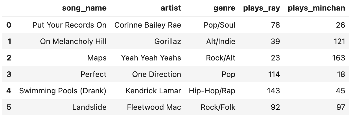
Ray and Minchan have a joint playlist that combines all songs they both listened to in the past month. Each row in the songs DataFrame represents a song in the playlist. The columns are: song_name (str), artist (str), genre (str), as well as two columns for the amount of times either has played each song, plays_ray (int) and plays_minchan (int). Below are the first six rows of songs, though there are many more entries.

Problem 1

Minchan wants to see his listening trends. Suppose he takes many samples of size 30 from plays_minchan and computes their means. For each statement below, select the best answer.

Problem 1.1

(a) We expect that at least 75% of all of the sampled values of plays_minchan lie within 2 standard deviations of the population mean.

• Yes, due to CLT

• Yes, due to Chebyshev’s

• No, due to CLT

• No, due to Chebyshev’s

• Yes, but for reasons that have nothing to do with Chebyshev’s or the CLT

• No, but for reasons that have nothing to do with Chebyshev’s or the CLT

Problem 1.2

(b) We expect that approximately 95% of all sample means lie within 2 standard errors of the population mean.

• Yes, due to CLT

• Yes, due to Chebyshev’s

• No, due to CLT

• No, due to Chebyshev’s

• Yes, but for reasons that have nothing to do with Chebyshev’s or the CLT

• No, but for reasons that have nothing to do with Chebyshev’s or the CLT

Problem 1.3

(c) Now assume the distribution of plays_minchan is right-skewed but with no outliers. Which of the following statements is true about these statistics of plays_minchan?

• The median is always greater than the mean

• The mean is always greater than the median

• The mean is usually greater than the median, but not always

• The median is usually greater than the mean, but not always

Problem 1.4

(d) If both Minchan’s and Ray’s plays distributions are normal, will the distribution formed by pooling both of their plays into one combined dataset be approximately normal?

• Always

• Sometimes

• Never

Problem 2

Select all sampling methods below where the resulting sample is an SRS of 20 songs from the songs DataFrame.

• Use songs.sample(20, replace=1)

• Use np.random.multinomial(20, np.ones(songs.shape[0]) / songs.shape[0]) to decide how many times to take each row for a sample.

• np.random.choice(songs.get("song_name"), 20)

• Randomly pick 20 genres without replacement, then within each picked genre, randomly pick a song.

• Randomly pick 20 artists without replacement, then within each picked artist, randomly pick a song.

• None of the above.

Problem 3

Problem 3.1

(a) Suppose Ray collected an SRS of the whole playlist (of an unspecified size), storing it in DataFrame ray_playlist. Complete the code below to bootstrap for an 80% confidence interval for the mean:

boot_means = np.array([])
for i in range(1000):
    sim = ray_playlist.___(a)___.get("plays_ray").mean()
    boot_means = np.append(boot_means, sim)

left = np.percentile(boot_means, ___(b)___)
right = np.percentile(boot_means, ___(c)___)

(a):

Problem 3.2

(b):

Problem 3.3

(c):

Problem 3.4

(b) After generating 1000 bootstrap means from ray_play, what does the distribution of boot_means approximate?

• The sampling distribution of the sample mean of plays by Ray

• The population distribution of plays by Ray

• The empirical distribution of plays by Ray

• The probability distribution of plays by Ray

Problem 3.5

(c) Which statements are correct about the 80% bootstrap confidence interval of the population mean that Ray just computed?

• 80% of songs have a number of plays by ray that lies within the interval.

• There is a 80% probability that the true mean lies in this interval.

• 80% of such intervals created from repeating the bootstrap process with new samples will contain the true mean.

• 80% of the bootstrap means lie in the interval.

Problem 4

Problem 4.1

(a) Ray calculated a 95% CLT-based confidence interval for the population mean of his number of plays per song, spanning [60.5, 100.5]. If the sample size used to construct the interval was 25 songs, what is the standard deviation of Ray’s plays?

Note: “Not enough information” is also a possible answer.

Problem 4.2

(b) If Ray increases the sample size from 25 songs to 100 songs, how does the width of his 95% CLT-based confidence interval change?

• Doubles

• Halves

• Becomes 1/4 as wide

• Stays the same

Problem 4.3

(c) Now Ray is curious about other confidence intervals he could have constructed. Given stats.norm.cdf(1.75) = 0.96, calculate the endpoints of a 92% CLT-based confidence interval.

Note: “Not enough information” is also a possible answer.

Problem 4.4

(d) Ray then constructs a 99% CLT-based confidence interval. Select all the cases that could be possible when comparing his new 99% CI to his original 95% CI.

• 99% CI is wider than 95%

• 99% CI is smaller than 95%

• They have the same width

👋 Feedback: Find an error? Still confused? Have a suggestion? Let us know here.