← return to practice.dsc10.com

This quiz was administered in-person. Students were allowed a double-sided sheet of handwritten notes. Students had 30 minutes to work on the quiz.

This quiz covered Lectures 17-21 of the Winter 2026 offering of DSC 10.

Note (groupby / pandas 2.0): Pandas 2.0+ no longer silently drops columns that can’t be aggregated after a groupby, so code written for older pandas may behave differently or raise errors. In these practice materials we use .get() to select the column(s) we want after .groupby(...).mean() (or other aggregations) so that our solutions run on current pandas. On real exams you will not be penalized for omitting .get() when the old behavior would have produced the same answer.

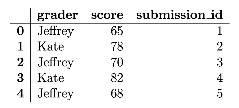
We are using (fictional) grading data from Quiz 3. Jeffrey and Kate each graded a random sample of DSC 10 submissions. The grading DataFrame has one row per graded submission with 50 rows total (25 per grader). The columns are: "grader" (str, either "Jeffrey" or "Kate"), "score" (int, score between 0 and 100), and "submission_id" (int, unique ID). The first few rows of grading are shown below.

After examining the difficulty of the last DSC 10 quiz, expert detective and professor Peter has deduced that one of the two graders has been grading significantly harsher than the other.

Problem 1

Using his years of statistical skill and investigative prowess, Detective Peter decides to conduct a permutation test to determine whether one of the two graders was significantly harsher than the other. He has Jeffrey’s scores and Kate’s scores and no assumed knowledge of the population distribution of scores. Which of the following best explains both why a permutation test is appropriate here and how it should be done?

• We have two samples and want to test whether they came from the same distribution. Under the null hypothesis, we simulate by shuffling the group labels, since if the distributions are the same the labels shouldn’t matter.

• We have two samples and want to test whether they came from the same distribution. Under the null hypothesis, we simulate by resampling with replacement from the combined 50 scores to form two new groups.

• We want to compare Jeffrey’s scores against a known population distribution of Quiz 3 scores. Under the null hypothesis, we simulate by shuffling scores and recomputing the test statistic.

• Shuffling the grader labels generates two new random samples from the population of all possible Quiz 3 scores, letting us estimate the sampling distribution of the test statistic.

Problem 2

Detective Peter moves forward with his permutation test to compare Jeffrey’s and Kate’s scores. He suspects that Jeffrey is the harsher grader — that is, Jeffrey’s scores tend to be lower than Kate’s, and wants to determine if there is evidence to support this.

Problem 2.1

Which null and alternative hypothesis pair is most appropriate?

• Null: Jeffrey and Kate gave scores from the same distribution. Alt: Jeffrey gave scores from a distribution with a smaller mean than Kate’s.

• Null: Jeffrey’s scores come from a known population with mean 70. Alt: Jeffrey’s scores do not come from a population with mean 70.

• Null: Jeffrey and Kate gave scores from the same distribution. Alt: The distribution of Jeffrey’s scores is entirely lower than the distribution of Kate’s scores.

• Null: The mean score from Jeffrey equals the mean score from Kate. Alt: The mean score from Jeffrey does not equal the mean score from Kate.

Problem 2.2

For testing whether Jeffrey is the harsher grader, which of the following could be used as a test statistic to get a p-value directly from its empirical distribution under the null hypothesis? Select all that are correct.

• The difference in group means: Kate’s mean minus Jeffrey’s mean.

• The difference in group means: Jeffrey’s mean minus Kate’s mean.

• The absolute difference between the two groups’ mean scores.

• The total variation distance between the two graders’ score distributions.

• None of the above.

Problem 3

Detective Peter asks another staff member, Ray, to write code to run the permutation test with 10,000 permutations. Ray comes up with his own test statistic and writes the following code to calculate an observed statistic, stored in observed_stat. Ray also wrote code (not shown) to store 10,000 simulated test statistics, each calculated in a manner matching the code for the observed statistic, in the array called simulated_stats. Fill in the two blanks below so it correctly computes the p-value for testing whether Jeffrey is the harsher grader.

observed_stat = (abs(grading[grading.get('grader') == 'Kate']
    .get('score').mean())
    - abs(grading[grading.get('grader') == 'Jeffrey']
    .get('score').mean()))

p_value = (simulated_stats ___(a)___ observed_stat).sum() / ___(b)___

Problem 3.1

(a)

Problem 3.2

(b)

Problem 4

After finding out through his expertly constructed permutation test that Jeffrey did, in fact, grade significantly harder than Kate, Detective Peter resolves to estimate the proportion of Jeffrey’s graded submissions that received a score below 70. He will construct a 95% CLT-based confidence interval for this proportion.

Problem 4.1

(a) He wants the confidence interval to have width at most 0.08. What is the minimum number of Jeffrey’s submissions he needs?

Problem 4.2

(b) Suppose he instead wants the width to be at most 0.04. The minimum sample size for that width is how many times the minimum sample size from part (a)?

Problem 5

Jeffrey frantically defends himself by claiming that the true proportion of his submissions that scored below 70 is really 0.20 — not nearly as bad as it looks! To test his claim, Detective Peter constructs a 95% confidence interval and gets [0.14, 0.40].

Problem 5.1

Using this confidence interval, at the 5% significance level, what decision should we make with respect to Jeffrey’s claim? Select all that are correct.

• Reject

• Fail to reject

• Accept

• Not enough information

Problem 5.2

Which of the following best explains why we reach that conclusion?

• Because 0.20 lies inside the confidence interval, the data are consistent with Jeffrey’s claim.

• Because 0.20 lies inside the confidence interval, the data are inconsistent with Jeffrey’s claim.

• Because the interval has a width of 0.26 which is much wider than we wanted, we do not have enough precision to reject any claim at the 5% significance level.

• Because the midpoint of the interval is 0.27, we have evidence against Jeffrey’s claim.

Problem 6

Overall, Detective Peter determined that Jeffrey’s offenses are grave enough: Peter travels all the way back to Tutorlandia to consult the great council of tutors on what Jeffrey’s penance should be. It was decided that Jeffrey must explain to the class what the total variation distance (TVD) measures. Which of the following is a correct description of the TVD?

• The difference between two group means.

• A measure of how different two distributions (of any type) are.

• A measure of how different two numeric distributions are.

• A measure of how different two categorical distributions are.

• The proportion of simulated statistics that are at least as extreme as the observed value.

• The width of a 95% confidence interval.

👋 Feedback: Find an error? Still confused? Have a suggestion? Let us know here.